
Full Terms & Conditions of access and use can be found at
https://www.tandfonline.com/action/journalInformation?journalCode=nurw20
Urban Water Journal
ISSN: (Print) (Online) Journal homepage: https://www.tandfonline.com/loi/nurw20
Prioritizing inspection of sewer pipes based on
self-cleansing criteria
Sergio Vanegas, Carlos Montes & Juan Saldarriaga
To cite this article:
Sergio Vanegas, Carlos Montes & Juan Saldarriaga (2022): Prioritizing
inspection of sewer pipes based on self-cleansing criteria, Urban Water Journal, DOI:
10.1080/1573062X.2022.2035408
To link to this article: https://doi.org/10.1080/1573062X.2022.2035408
Published online: 13 Feb 2022.
Submit your article to this journal
Article views: 41
View related articles
View Crossmark data

RESEARCH ARTICLE
Prioritizing inspection of sewer pipes based on self-cleansing criteria
Sergio Vanegas
, Carlos Montes
and Juan Saldarriaga
Department of Civil and Environmental Engineering, Universidad de Los Andes, Bogotá, Colombia
ABSTRACT
This paper aims to develop a sediment deposits hydraulic deterioration model based on self-cleansing
criteria to prioritize the inspection of sewer systems. The model was trained with benchmarking literature
values from earlier experiments and validated with household connections complaints data from Bogotá,
Colombia. Recursive Feature Elimination with Cross-Validation (RFECV) and Bayesian Optimization (BO)
were used to construct a Random Forest (RF) model to predict, at pipe level, the likelihood for a pipe to
present sediment deposits. To evaluate the model’s prediction accuracy, two different performance
indicators were used: (i) the Percentage of Effective Inspections, and (ii) Pipes per Inspection with
sediments. The sediment deposits hydraulic deterioration model shows good overall performance with
buffer zones radiuses of 250 m predicting which pipes tend to present sediment deposits over time. This
model improves the understanding of sediment deposits in hydraulic deterioration models and can be
used to prioritize inspection of sewer systems.
ARTICLE HISTORY
Received 18 March 2021
Accepted 24 January 2022
KEYWORDS
Urban drainage; data
management; non-cohesive
sediment transport; self-
cleansing sewer pipes
Introduction
Sewer systems performance is a constant challenge for water
utilities, due to the changing environment and the low flexibility
in space for infrastructure associated with constraints in terrain
gradients and fixed locations (Tscheikner-Gratl et al.
2019
). As
a result, collecting information from sewer systems is both
expensive and time-consuming for water utilities (Hahn et al.
2002
; Elmasry, Zayed, and Hawari
2018
). Those utilities have
traditionally addressed the inspection of sewer systems with
a reactive approach (Ariaratnam, El-Assaly, and Yang
2001
;
Rodríguez et al.
2012
) or a poor proactive approach (Tscheikner-
Gratl et al.
2019
), which represent an inefficient expend of limited
funds. Consequently, prioritizing inspection with available data
from sewer systems is important for a cost-effective strategy to
ensure the network is functioning appropriately.
To address this issue, several authors have developed struc-
tural and hydraulic deterioration models for sewer systems.
Structural deterioration models (Ariaratnam, El-Assaly, and
Yang
2001
; Tran, Ng, and Perera
2007
; Zhou et al.
2008
;
Harvey and McBean
2014
; Caradot et al.
2017
; Yin et al.
2020
)
are more common and are related to structural defects, such as
surface damage, cracks and fractures. Hydraulic deterioration
models are commonly used to complement structural dete-
rioration models (Hahn et al.
2002
; Berardi et al.
2008
; Hawari
et al.
2017
; Elmasry, Hawari, and Zayed
2017
; Elmasry, Zayed,
and Hawari
2018
; Daher et al.
2018
; Ghavami, Borzooei, and
Maleki
2020
). The latter are related to operational defects, such
as infiltration, soil intrusion, tree root intrusion and sediment
deposits, which reduce the hydraulic capacity of sewer pipes. In
general, structural and hydraulic deterioration models are used
in asset management to prioritize inspection of sewer systems
to ensure acceptable network performance.
Existing models can be classified, according to their model-
ling technique, into three categories (Tscheikner-Gratl et al.
2019
): (i) deterministic, (ii) statistical and (ii) Artificial
Intelligence (AI) models. Deterministic models aim to under-
stand the physical mechanisms leading to pipe deterioration,
which implies the collection of accurate data under controlled
environments for measuring specific variables. Statistical mod-
els require less precise information as they define the model
structure, in terms of input variables processing, prior to train-
ing. AI models can determine complex interactions between
variables without making assumptions (Tran
2007
), which tends
to increase their predictive capacity. Most authors have built
statistical or AI models using information related to historical
pipe performance, which is usually collected and stored by
water utilities through closed-circuit television (CCTV)
inspections.
In general, sewer pipe deterioration is a continuous process
affected by several aspects that are difficult to measure in
practice. This makes the development of deterioration models
a challenging task. Most of the models developed have been
trained with historical data collected by water utilities, which
makes them rely on the frequency and distribution of past
events. As the training data of the models is based on historical
events, their performance does not depend on the complete
understanding of the deterioration phenomena (Rodríguez
et al.
2012
). In contrast, model accuracy is directly dependent
on the quality of historical data collected in-situ. Usually, these
deterioration models tend to show poor generalisation and
extrapolation capabilities, i.e. accuracy is quickly lost when
applied to external datasets (Tscheikner-Gratl et al.
2019
). As
a result, existing models can only be used in the sewer system
of the site where the data was collected.
CONTACT
Juan Saldarriaga
jsaldarr@uniandes.edu.co
URBAN WATER JOURNAL
https://doi.org/10.1080/1573062X.2022.2035408
© 2022 Informa UK Limited, trading as Taylor & Francis Group

To address this issue, specifically the poor generalisation of
models, benchmarking experimental data is used for modelling
sediment deposits that contributes to the process of hydraulic
deterioration. This operational defect is one of the most com-
mon hydraulic challenges in sewer systems, which can form
blockages that reduce the pipes’ hydraulic capacity and may
cause premature overflows (Tran
2007
; Banasiak
2008
;
Rodríguez et al.
2012
; Elmasry, Hawari, and Zayed
2017
;
Montes, Kapelan, and Saldarriaga
2019
). As an example,
Rodríguez et al. (
2012
) found that 54% of effective sediment-
related failures (effective blockages) in Bogotá, Colombia, were
related to sewer pipes; the other 24% and 22% of effective
blockages were related to gully pots and manholes, respec-
tively. Based on this, the development of a tool to prioritize the
inspection of sediment deposits in pipes is important to pre-
vent uncontrolled hydraulic deterioration due to this opera-
tional defect.
This paper seeks to develop a sediment deposits hydraulic
deterioration model based on non-deposition sediment trans-
port concepts to prioritize the inspection of sewer systems.
Experimental data of non-deposition without deposited bed
and non-deposition with deposited bed was collected from
literature to train a model that computes the likelihood of
both conditions. This approach permitted predicting the like-
lihood of a pipe having sediment deposits under different
hydraulic conditions as the non-deposition with sediment bed
condition is near the condition where permanent sediment
deposits are formed. To measure the predictive capacity
under pragmatic conditions to emulate the normal operation
of a system, the model was implemented in one zone of the
stormwater sewer system in Bogotá, Colombia. The aim is to
improve the understanding of sediment deposits in hydraulic
deterioration models and to use this knowledge to prioritize
the inspection of sewer systems. In general, the developed
model can show water utilities which areas they should have
under supervision according to their inspections and different
hydraulic conditions.
Methodology
Self-cleansing criteria concepts
To improve the understanding of sediment deposits in hydrau-
lic deterioration models, non-deposition sediment transport
concepts were used. This field of research has been studied
by several authors (Ab Ghani
1993
; Vongvisessomjai,
Tingsanchali, and Babel
2010
; Ebtehaj and Bonakdari
2016
;
Montes et al.
2020a
,
2020b
) who have developed regression-
based models using experimental data collected at laboratory
scale, to describe the behaviour of particles under certain flow
conditions, especially under steady flow conditions. In general,
Robinson and Graf (
1972
) identified two flow regimes: (i) non-
deposition and (ii) deposition. The threshold between both
flow regimes is determined by the critical velocity, which is
related to the critical condition where particles begin to form
a transitional bed at the bottom of the pipe. As these deposits
reduce the hydraulic capacity of pipes, sewer systems are com-
monly designed under the non-deposition regime, where flow
velocities are higher than the critical velocity. This flow regime
has been classified into two subgroups (Safari, Mohammadi,
and Ab Ghani
2018
): (i) non-deposition without deposited bed
and (ii) non-deposition with deposited bed.
The first group, non-deposition without deposited bed, is
a conservative approach for designing self-cleansing sewers in
which sediment particles move separately and slowly at the
bottom of the pipe, i.e. without forming a permanent or
a transitional sediment deposit bed. Several authors (Mayerle
1988
; Ab Ghani
1993
; May
1993
; Vongvisessomjai, Tingsanchali,
and Babel
2010
; Montes et al.
2020a
,
2020b
) have studied these
conditions to predict the minimum self-cleansing velocity for
this flow regime. In general, these studies carried out extensive
experimental research varying both sediment and flume/pipe
properties, as shown in
Table 1
. With the data collected, several
regression-based models to predict the sediment velocity that
generates non-deposition without sediment bed conditions
were developed.
The second group is less conservative and allows
a transitional deposited loose bed as bedload. Several authors
(May et al.
1989
; El-Zaemey
1991
; Ab Ghani
1993
; Butler, May,
and Ackers
1996
) have found that a mean proportional sedi-
ment depth (y
s
=
D) close to 1.0% of the pipe diameter, increases
the sediment transport capacity. In contrast to non-deposition
without deposited bed, this flow regime is near the critical
condition, and regular supervision of the systems is required
for preventing the formation of permanent sediment deposits
(Vongvisessomjai, Tingsanchali, and Babel
2010
). In this con-
text, several studies (Perrusquia
1991
; El-Zaemey
1991
; Ab
Ghani
1993
; Montes et al.
2020b
) carried out at laboratory
scale have studied this sediment transport mode varying the
inlet conditions, as seen in
Table 1
. In the same manner, these
studies developed different models to predict the sediment
velocity under different hydraulic conditions and sediment
characteristics that generate non-deposition with sediment
bed conditions.
In general, non-deposition without deposited bed and non-
deposition with deposited bed have been studied indepen-
dently at laboratory scale as they are two different approaches
for designing self-cleansing sewer pipes. Nevertheless, there is
no quantitative threshold between these subgroups since the
transition between them is almost imperceptible and requires
complete knowledge of the phenomena to be able to identify
it. In this study, as there is no numerical expression for this limit,
the data-driven Random Forest (RF) technique is used to pre-
dict the likelihood of each flow regime (i.e. non-deposition
without deposited bed and non-deposition with sediment
bed) under different flow conditions. As the non-deposition
with deposited bed criteria is near the critical condition where
stationary deposits are formed, this classification model can be
used to develop a sediment deposits hydraulic deterioration
model that, combined with Geographic Information Systems
(GIS) can be implemented to prioritize the inspection of sewer
systems. More details of the implementation are given below.
Literature data
Literature data for both non-deposition conditions were col-
lected to train the RF model.
Table 1
is modified from Montes,
Kapelan, and Saldarriaga (
2021
) and summarize this
information.
2
S. VANEGAS ET AL.

As shown in
Table 1
, results from 541 and 408 tests were
collected for non-deposition without deposited bed and non-
deposition with deposited bed, respectively. In general, the
following input variables were obtained for each test: d the
mean particle diameter, SG the specific gravity of the sedi-
ment, S
o
the pipe slope, D the pipe diameter, Y the water
level, R the hydraulic radius, V the flow velocity, λ the Darcy
friction factor, and C
v
the volumetric sediment concentration.
Then, additional parameters such as, D
gr
the dimensionless
grain size and τ the shear stress were computed. The initial
training dataset has 949 reference values collected from the
literature. However, as the training dataset only considers
a limited number of combinations between hydraulic condi-
tions, pipe characteristics and sediment properties, its size
directly affects the capabilities of extrapolation for
a Machine Learning (ML) model. Models’ performance tend
to increase with more data, but more data does not always
imply an increase in performance; the quality of additional
data and data pre-processing are equally important (Zhu et al.
2016
).
To address this issue, data augmentation based on physical
knowledge of non-deposition flow regimes was used to gen-
erate new records. The above means that new records were
created based on the known physical principles of non-
deposition flow regimes. The parameters that were constant
through this procedure were D, S
0
and C
v
, while the filling ratio
of the pipe and the sediment characteristics varied. These two
parameters were varied because during experimental test col-
lection in the study of Montes et al. (
2020b
), it was observed
that certain changes in both parameters do not affect the non-
deposition flow regime. The non-deposition without deposited
bed condition is preserved when the filling ratio changed from
the observed value in the experimental test until it reached
85% with interval increases of 1% and with all the particles with
lower mean diameter from the observed. The non-deposition
with deposited bed condition is preserved when the filling ratio
changed from the observed value in the experimental test until
it reached 1% with interval decreases of 1% and with all the
particles with greater mean diameter from the observed. The
above was considered since this behaviour was observed dur-
ing the experiments carried out by the authors in previous
research (Montes et al.
2020a
,
2020b
). With this approach,
454,595 different combinations of parameters were obtained
to train the model.
Sediment deposits hydraulic deterioration model
RF is a supervised ML algorithm proposed by Breiman (
2001
)
which consists of a combination of decision trees, where each
tree is generated from identically distributed random vectors.
These vectors are used to select training samples and input
variables for each tree. With this approach, an ensemble of
decision trees is generated, where each tree computes the
output variable and the result is given by the average of all
the ensemble (James et al.
2013
). This procedure allows RF to
find non-linear relations between variables and reduce model
variance. However, RF performance is directly dependent on
the input variables and the definition of the hyperparameters
(e.g. maximum node depth and the number of trees, among
others). To overcome these issues, Recursive Feature
Elimination with Cross-Validation (RFECV) and Bayesian
Optimization (BO) were used, respectively. Then, the Receiver
Operating Characteristic (ROC) curve was constructed to deter-
mine the likelihood cut-off (threshold for classification). Finally,
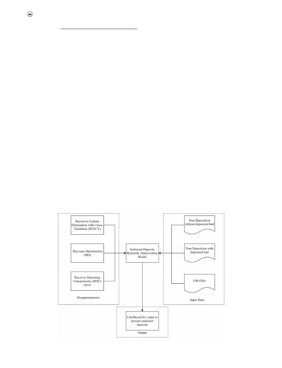
the obtained RF model was integrated with GIS tools, such as:
feature selection, buffer analysis, intersect analysis, feature
layer creation, spatial join, and mapping.
Figure 1
shows the
implementation of the hydraulic deterioration model devel-
oped here. More details of the methods used are described
below.
RFECV is a combination of Recursive Feature Elimination
(RFE) and Cross Validation (CV). RFE is a greedy search back-
ward selection method that was introduced by Guyon et al.
(
2002
) to improve the selection of input variables and reduce
computational costs associated with this process. In general,
this algorithm trains a classifier, then computes a scoring metric
for each input variable and finally removes the least important
one. This method was then combined with a CV resampling
method, which allows the creation of training and testing sub-
sets for each RFE iteration. Specifically, Stratified K Fold CV with
k ¼ 3 was used for this procedure, which divides the original
data in three subsets, including training, testing, and preserving
the percentage of samples for each class. The accuracy CV score
defined in Equation (1) was selected as scoring metric. Since the
RF model predicts the likelihood of non-deposition without
deposited bed and non-deposition with sediment bed under
different flow conditions, a prediction is considered correct
when a certain flow condition of the testing subset is classified
according to the likelihood cut-off (threshold for classification)
in the same flow regime as claimed in the testing subset.
Table 1.
Collected experimental data.
Reference
Non-deposition criterion
No. of tests
Pipe diameter (mm)
Particles diameter (mm)
Pipe slope (%)
Water level (mm)
Mayerle (
1988
)
Without deposited bed
106
152
0.50–8.74
0.14–0.56
28–122
May (
1993
)
Without deposited bed
27
450
0.73
0.04–0.30
222–338
Ab Ghani (
1993
)
Without deposited bed
221
154, 305 and 405
0.46–8.30
0.04–2.56
23–338
Vongvisessomjai, Tingsanchali,
and Babel (
2010
)
Without deposited bed
36
100 and 150
0.20–0.43
0.20–0.06
20–60
Montes et al. (
2020a
)
Without deposited bed
44
242
1.33–1.51
0.2–0.8
24–161
Montes et al. (
2020b
)
Without deposited bed
107
595
0.35–2.6
0.04–3.43
11–218
Perrusquia (
1991
)
With deposited bed
38
225
0.9
0.02–0.06
23–115
El-Zaemey (
1991
)
With deposited bed
290
305
0.53–8.40
0.18–0.44
39–203
Ab Ghani (
1993
)
With deposited bed
26
450
0.73
0.07–0.47
204–345
Montes et al. (
2020b
)
With deposited bed
54
595
0.47–2.60
0.46–5.42
14–91
URBAN WATER JOURNAL
3
Accuracy CV score ¼
Correct predictions in test dataset
Total number of predictions in test dataset
(1)
For this process, the RF was trained with 100 trees with the Gini
Impurity index as the main criterion for measuring the quality of
a split and with no restriction over the maximum depth. The
Python library scikit-learn (Pedregosa et al.
2015
) was used for
implementing RFECV and RF algorithms.
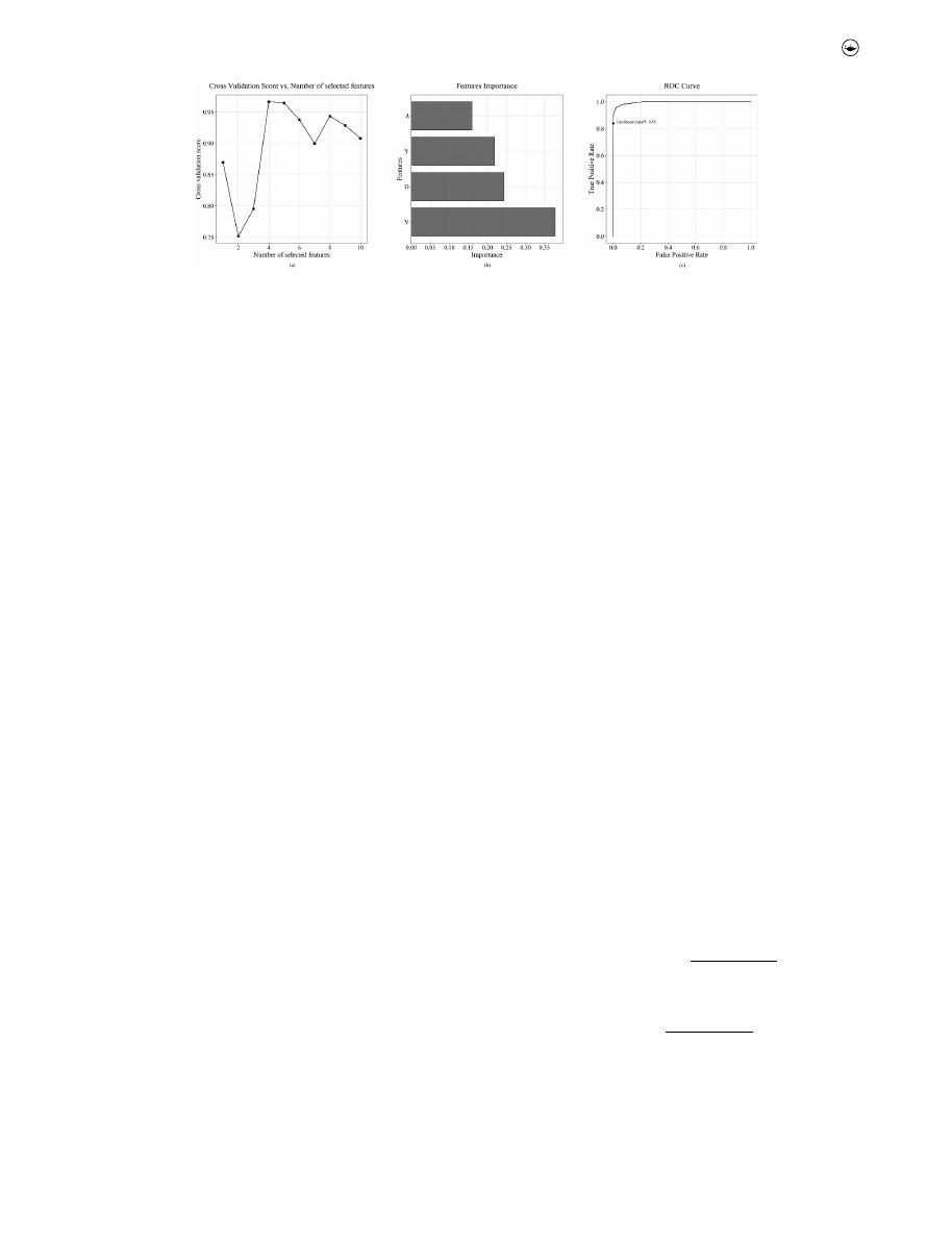
Figure 2(a
) shows the
accuracy CV score for each number of selected features in RFECV,
the possible features for the model were: d, SG, S
o
, D, Y, R, V, λ, D
gr
and τ. The highest CV score was obtained for four selected
features: D, Y, V and λ.
Figure 2(b
) shows the importance of the
selected features, computed with the Gini Impurity Index. As
shown in this figure, the most important features are the flow
velocity, i.e. the mean velocity of the pipe computed with the
filling ratio and the Darcy Weisbach – Colebrook White coupled
equation for part-full flow, and the pipe diameter, respectively.
BO is a sequential optimization method that commonly uses
Gaussian Processes (GP) to fit an unknown objective function
(Wang et al.
2016
). BO uses GP approximation to lead explora-
tion of solution space for areas that are expected to give more
information about the solution space, which is then used to
update the distributions of the approximated objective func-
tion (Garrido-Merchán and Hernández-Lobato
2020
). As the
objective function for RF hyperparameter tuning is an unknown
non-convex function, BO is used for selecting the hyperpara-
meters. For this process, the RF algorithm was trained with the
input variables obtained from RFECV. Additionally, RF hyper-
parameters and their space of solutions were defined as fol-
lows: (i) number of trees, integer solution between 100 and 400;
and (ii) maximum depth, integer solution between 3 and 10.
The Python libraries scikit-learn (Pedregosa et al.
2015
) and
scikit-optimize (Head et al.
2018
) were used for implementing
RF algorithm and BO, respectively. For the BO process, 5 ran-
dom starts, 15 iterations and accuracy as metric were defined as
parameters. The obtained hyperparameters were: (i) number of
trees equivalent to 400 and (ii) maximum depth of 5.
ROC curve is a graphical analysis tool that plots the relation-
ship between true positive rate (TPR) and false-positive rate
(FPR) for a classification model considering different likelihood
cut-offs.
Figure 2(c
) shows the ROC curve for the RF model
using the input variables from the RFECV and the hyperpara-
meters from BO. This analysis is used to select the likelihood
cut-off that best fits the model requirements. This value will be
used as the threshold for the classification in the RF model. As
predicting false positives pipes is associated to an inefficient
use of funds, a likelihood cut-off of 0.55 is selected, with a TPR
of 0.839 and a FPR of 0.000.
The obtained RF model is integrated with GIS tools to obtain
the sediment deposits hydraulic deterioration model. In gen-
eral, this process is made using arcpy Python library from
ArcGIS, which allows to integrate GIS files and use them as
input for the classification model. Additionally, the predictions
made with the RF model are integrated with two GIS features:
the network connectivity matrix and buffer zones. The network
connectivity matrix makes possible the consideration of pipes
surroundings at underground level. This is important for the
sediment deposits predictions, as this operational defect
reduces the hydraulic capacity of a pipe, which directly affects
adjacent pipes. Buffer zones are used to delimit the influence
area of water utilities inspections, which permits the model to
have real-time data of the pipes that can present sediment
deposits and those that have been recently inspected. Using
Figure 1.
Sediment deposits hydraulic deterioration model development.
4
S. VANEGAS ET AL.
this approach, the likelihood of a pipe having sediment depos-
its under different hydraulic conditions can be predicted at
pipe level.
Discrete dynamic simulation and performance measures
A discrete dynamic simulation was built to evaluate the
model performance over time. This discrete dynamic simu-
lation consisted of integrating the RF model with GIS tools
to simulate the network sediment deposits state at pipe
level by days. For this process, the following parameters
were defined: (i) starting date, (ii) number of time steps,
(iii) timesteps for the RF model, (iv) radiuses of the buffer
zones for inspections that are used to create areas in which
inspections are considered effective (i.e. an inspection in
which sediment deposits have been found), (v) maintenance
time frame for inspections that defines the number of time-
steps in which the buffer zone of an inspection is active,
which means that the pipes within the buffer zone are not
considered as candidates for developing sediment deposits
during this time frame, (vi) sediment deposits likelihood
increasing factor that emulates the reduction in the hydrau-
lic capacity pipes caused by physical impact of sediment
deposits in adjacent pipes. For example, an increasing factor
of 1.10 means that the likelihood of developing sediment
deposits is 10% higher than otherwise and (vii) performance
measures for each timestep of the simulation.
For each day in the simulation time, the sediment deposits
hydraulic deterioration model verifies which inspections were
made by the Empresa de Acueducto y Alcantarillado de Bogotá
(EAB), and creates a buffer zone around records for that
specific day with a defined radius and a maintenance time
frame. During this time frame, the buffer zone is active which
means he pipes within this area are not considered for the
prediction of the state for sediment deposits. In general, these
predictions are made under random hydraulic conditions, gen-
erated specifically with a random filling ratio, where the like-
lihood of a pipe to have sediment deposits is computed every n
timesteps. The likelihood is affected by an increasing factor
which is computed only if the pipe that is being simulated
has an adjacent pipe with sediment deposits according to the
model. If the RF model classifies the state of a pipe as ‘with
sediment deposits’, this state is preserved until the pipe is
inspected. A pipe is inspected once it is within a buffer zone
of an inspection. Additionally, for each day the following out-
puts are computed according to the starting date (t) and num-
ber of days that the simulation has been running (δ):
●
Total Inspections (TI
t;tþδ
): Defined as the total number of
registered inspections from t to t þ δ.
●
Failed Inspections (FI
t;tþδ
): Defined as the total number of
failed inspections from t to t þ δ. An inspection is consid-
ered as non-satisfactory if there are no pipes with sedi-
ment deposits within the radius of the defined buffer
zone, which means that the inspection made by the
water utility did not found any pipe that needed to be
cleansed. It is important to point out that the simulations
works only with inspections related with the cleansing of
the stormwater sewer system.
●
Pipes with sediments confirmed by inspection (IP
t;tþδ
):
Defined as the total number of inspected pipes with sedi-
ments from t to t þ δ. A pipe is considered with sediments
confirmed by inspection if it was within the defined buffer
zone radius with sediment deposits, which means that the
inspection made by the water utility found at least one pipe
that needed to be cleansed in the buffer zone.
With these outputs, the following performance measures for
each simulation day are defined to evaluate model’s prediction
accuracy: Percentage of Effective Inspections (PEI
t;tþδ
) and
Pipes per Inspection with sediments (PP
t;tþδ
). PEI
t;tþδ
quantifies
how many inspections were effective during the simulation,
while PP
t;tþδ
shows how many pipes could be cleansed by the
water utility by inspection with a defined buffer zone radius.
Equations (2) and (3) show these calculations, respectively:
PEI
t;tþδ
¼
100% �
TI
t;tþδ
FI
t;tþδ
TI
t;tþδ
(2)
PP
t;tþδ
¼
IP
t;tþδ
TI
t;tþδ
FI
t;tþδ
(3)
It is important to highlight that some of the outputs from the
performance measures depend directly on the buffer zones
radiuses. Therefore, the performance measures change when
the buffer zones radiuses is varied. In general, these measures
increase with increases in the buffer zones radiuses. However,
Figure 2.
Sediment deposits hydraulic deterioration model results. (a) Cross Validation Score according to the number of selected features, (b) The features importance
in the Random Forest model, and (c) The ROC curve for the model.
URBAN WATER JOURNAL
5
increases in the buffer zones radiuses can be related to less
accuracy in the model, because more area is needed to be
inspected for each inspection.
For the simulations, the selected starting date was 2019–09-
09; the total time of simulation were 200 days; the timesteps for
the RF model was 4 days; the maintenance time frame was
generated randomly for each register in the database of 61
registers related with the cleansing of the stormwater system
from a discrete cumulative probability distribution function
obtained from historical data; the buffer zones radiuses for
inspections was evaluated for 150 m, 200 m, and 250 m; and
the sediment deposits likelihood increasing factor was evalu-
ated for 1.10, 1.25 and 1.40. The defined performance measures
were obtained for each day with t ¼ 0 and δ equivalent to the
simulation day.
Case Study: Zone 1 Bogotá
In this study, the developed sediment deposits hydraulic dete-
rioration model was validated with data from the household
connections’ complaints database from Bogotá. The EAB
divides the sewer system of the city of Bogotá in five opera-
tional zones. Only Zone 1 was selected for validating the
hydraulic sediment deposits deterioration model. This zone
has about 597,592 household connections, 92% of them are
classified as residential and are distributed in an area of
approximately 177 km
2
.
The GIS geodatabase of the stormwater sewer system has
20,939 pipe sections with information of diameters, slopes,
materials, invert elevation, age, and length. The total pipe
length of the stormwater sewer system is 908 km. However,
some records had unknown or inconsistent information, e.g.
extremely steep or unknown slopes and/or extremely large or
unknown diameters. These pipes with missing data were elimi-
nated to prevent using unknown data during the simulations.
After data cleansing, 15,022 pipe sections were obtained for
validating the sediment deposit hydraulic deterioration model.
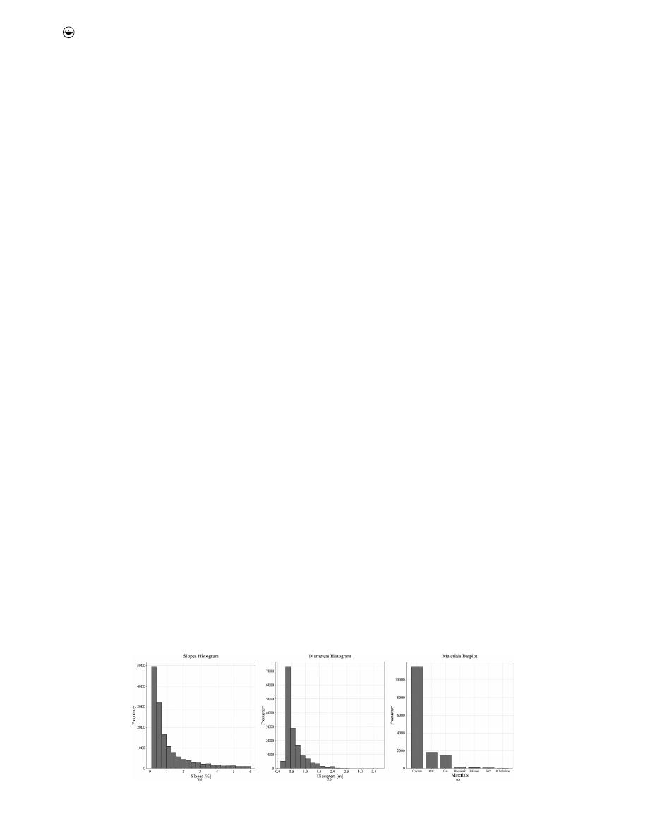
Figure 3(a
) shows the distribution of the pipe section slopes in
the network, which are mostly less than 1%. In total, 5917 were
not considered for the simulation, however they are distributed
along all the network and do not affect the general network
connectivity. Nevertheless, if in the future the model is going to
be implemented by a water utility, it is highly recommended to
have complete data for the simulated network.
Figure 3(b
)
shows the distribution of the pipe diameters in the system,
where most values range from 300 mm to 600 mm. Finally,
Figure 3(c
) shows the distribution of the pipe materials in the
stormwater sewer system, where the most common material
found is concrete, followed by PVC and clay.
For the case study, the EAB has two main record databases.
The first one has maintenance records of sanitary and storm-
water sewer pipes from 2008 to 2018, which are used to analyse
the behaviour of the network throughout time. The database
has 14,810 records associated to sewer cleansings between
2010 and 2018. These records were used to estimate the time
between inspections adjusting a discrete cumulative probabil-
ity distribution function for obtaining the maintenance time
frame for the simulation. The second database has 61 records
that are inspections related with the cleansing of the storm-
water sewer system. These inspections are made by visual
inspection as soon as possible, according to household con-
nections’ complaints. This database was used to test the model
developed here with the assumption that each record is an
inspection where the cleansing was effectively made. More
details about how this database information was used are
described in the section below.
Results and discussion
Results
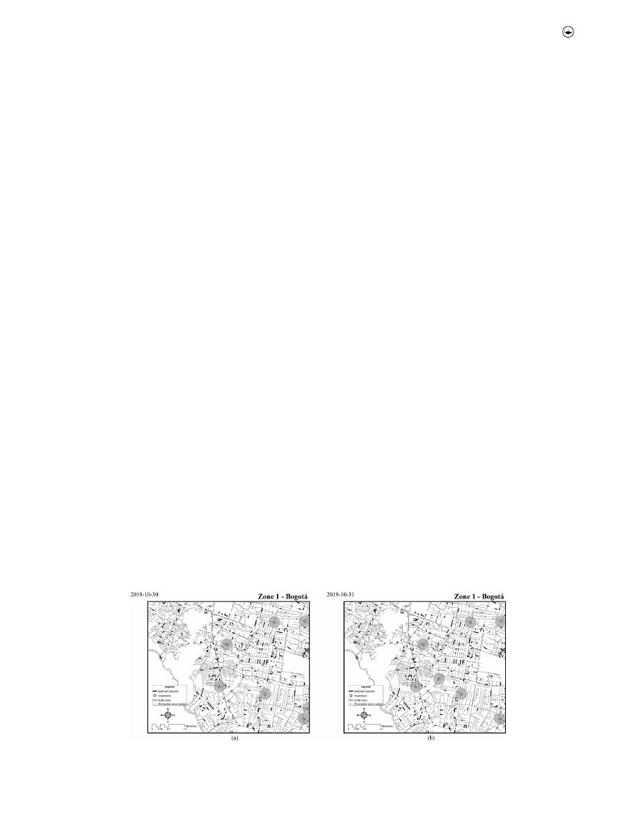
Figure 4
shows an example of the map results during the
discrete dynamic simulation for buffer zones radiuses of
250 m and the sediment deposits likelihood increasing factor
equivalent to 1.25. It is important to highlight that in the map
the pipes with sediment deposits are obtained according to the
model.
Figure 4(a
) shows a region of the case of study on
30 October 2019 where seven inspections are active (the time-
step is included during the maintenance time frame of the
inspections), which means the pipes within their buffer zones
are not considered as candidates for the prediction of the
deposition state.
Figure 4(b
) shows the same region the
next day, where seven inspections are active, but one of the
active inspections of the previous day was deactivated (the
maintenance time frame of this inspection ends) and a new
inspection became active. Comparing
Figure 4(a,b
), when the
new inspection is active in
Figure 4(b
) the pipes that the
deterioration model had identified in previous days with sedi-
ment deposits were cleansed. On the other hand, when the
other inspection was deactivated, the pipes within its buffer
zone are now considered by the deterioration model and
Figure 3.
Stormwater sewer system description plots. (a) Slopes Histogram, (b) Diameters Histogram, and (c) Materials Barplot.
6
S. VANEGAS ET AL.
sediment deposits are identified. Additionally, from
Figure 4
the impact of the likelihood increasing factor can be identified
as sediment deposits are usually identified on adjacent pipes.
Figure 5
was constructed with the values for the perfor-
mance measures for each day differentiating the values for
the buffer zones radiuses and the sediment deposits likelihood
increasing factor. The curves show the evolution of the perfor-
mance indicator over time. The expected behaviour is that
these indicators converge to one value over time.
Figure 5(a,
b)
are obtained for buffer zones radiuses of 150 m,
Figure 5(c,d
)
are obtained for buffer zones radiuses of 200 m and
Figure 5(e,
f
) are obtained for buffer zones radiuses of 250 m.
Figure 5(a,c
and e
) show the behaviour of PEI
t;tþδ
and
Figure 5(b,d and f
)
show the behaviour of PP
t;tþδ
, both for different values of the
sediment deposits likelihood increasing factor. The following
observations can be made from
Figure 5
:
●
The highest PEI
0;200
for all the buffer zones radiuses is
obtained with a sediment deposits likelihood increasing
factor of 1.25. The PEI
0;200
obtained values are 65%, 70%
and 83%; for 150 m, 200 m, and 250 m; respectively. While
the lowest PEI
0;200
for all the buffer zones radiuses is
obtained with a sediment deposits likelihood increasing
factor of 1.10. The PEI
0;200
obtained values are 62%, 68%
and 80%; for 150 m, 200 m, and 250 m; respectively.
●
For
Figure 5(a
) the PEI
0;200
for all increasing factors are
around 63%, for
Figure 5(c
) the PEI
0;200
for all increasing
factors are around 69% and for
Figure 5(e
) the PEI
0;200
for
all increasing factors are around 82%. As
Figure 5(a,c and
e
) are constructed with buffer zones radiuses of 150 m,
200 m and 250 m, increases of 5 m in the buffer zones
radiuses suggest an increase on average of 1% in PEI
0;200
.
●
The highest PP
0;200
for all the buffer zones radiuses is
obtained with a sediment deposits likelihood increasing
factor of 1.40. The PP
0;200
obtained values are 2.54 pipes,
4.22 pipes and 5.53 pipes; for 150 m, 200 m, and 250 m;
respectively. While the lowest PP
0;200
for all the buffer
zones radiuses is obtained with a sediment deposits like-
lihood increasing factor of 1.10. The PP
0;200
obtained
values are 2.14 pipes, 3.27 and 4.06; for 150 m, 200 m,
and 250 m; respectively.
●
For
Figure 5(b
) the PP
0;200
for all increasing factors are
around 2.35 pipes, for
Figure 5(d
) the PP
0;200
for all
increasing factors are around 3.81 pipes, for
Figure 5(f
)
the PP
0;200
for all increasing factors are around 4.83 pipes.
As
Figure 5(b,d and f
) are constructed with buffer zones
radiuses of 150 m, 200 m and 250 m, increases of 50 m in
the buffer zones radiuses suggest an increase on average
of 1.245 pipes in PP
0;200
.
Discussion
Considering the results presented in
Figures 4 and 5
, and their
respective observations, the following remarks are made:
●
As it was mentioned in the description of
Figure 4
, it is
pertinent to mention the importance of the likelihood
increasing factor.
Figure 4(a,b
) show that the deterioration
model tends to identify sediment deposits in adjacent pipes
due to the likelihood increasing factor. This is relevant for
the deterioration model because it emulates the reduction
in the hydraulic capacity pipes caused by sediment depos-
its. This operational defect directly affects adjacent pipes
and pushes toward the creation of more sediment deposits.
●
In
Figure 4(a,b
), it can be identified that some regions are
predisposed to present sediment deposits. This is caused
by two main aspects: (i) the likelihood increasing factor
and (ii) similarities in pipe characteristics. The first aspect
was discussed in the previous remark and contributes to
identifying some specific areas with sediment deposits.
The second aspect is more related to sewer design, where
in small regions similar pipes characteristics are chosen to
avoid flow disturbances. As similar pipe characteristics are
chosen, the obtained hydraulic conditions are also similar.
This implies that if a pipe tends to present sediment
deposits, another pipe with similar characteristics is also
likely to have this operational defect, which explains the
concentration of sediment deposits in some regions.
●
Figure 5
shows that the best overall results are obtained
with a buffer zones radiuses of 250 m and an increasing
factor of 1.25.
Figure 5
also suggest that if the buffer zones
radiuses is increased the performance measures will tend
Figure 4.
Map results example for buffer zone radius 250 m and likelihood increasing factor of 1.25. Stars, circles and wide lines denote the inspections, buffer zone
radius and pipes with sediment deposits, respectively. (a) Shows the simulation result on 2019–10-30, and (b) Shows the simulation result on 2019–10-31.
URBAN WATER JOURNAL
7
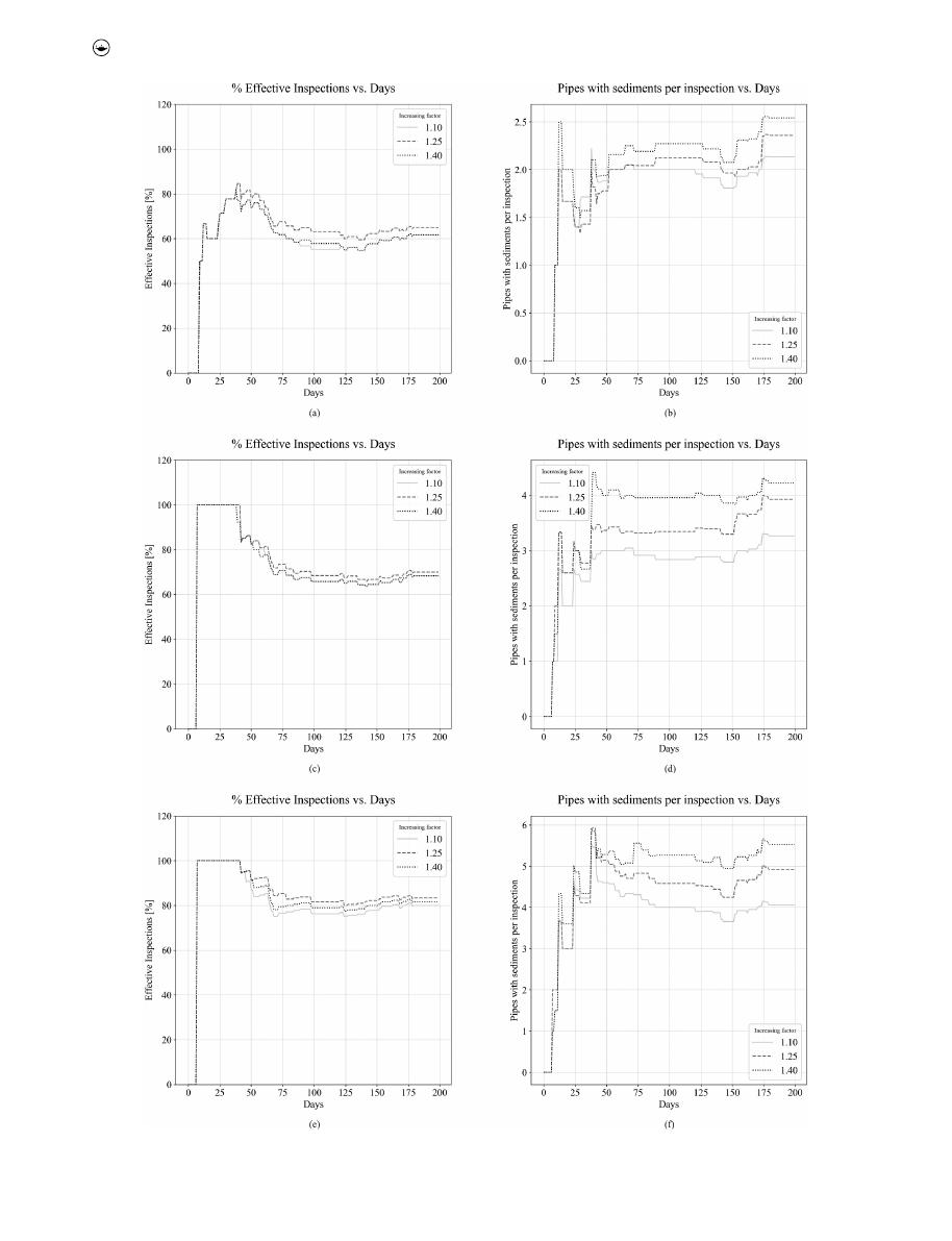
Figure 5.
Performance measures. a) and b) for buffer zone radius of 150 m, c) and d) for buffer zone radius of 200 m, e) and f) for buffer zone radius of 250 m.
8
S. VANEGAS ET AL.

to increase as well. However, it is desirable to make the
buffer zones radiuses smaller to obtain higher precision
for each inspection, which is associated with a better use
of water utilities funds.
●
The obtained sediment deposit hydraulic deterioration
model can be used in any sewer network with GIS infor-
mation, as it was trained with benchmarking experimental
data. This feature makes the model not dependent of any
sewer network, which fixes the poor generalisation and
extrapolation capabilities of other models. Nevertheless,
the historical data from the sewer networks can be used
to evaluate the model performance measures and assess
its precision in other sewer networks.
●
The sediment deposit hydraulic deterioration model can
be used by water utilities to prioritize the inspection of
sewer systems, as this model identifies regions that are
predisposed to deposition and updates its results based
on the water utilities operation.
●
Considering that predictions for each time step are made
under random hydraulic conditions, specifically a random
filling ratio, it is important to highlight the importance of
simulating multiple rounds, because this ensures that on
some rounds, the likely places of sedimentation will be
spotted by the model. For further research, the hydraulic
conditions can be complemented with hydrological models.
Conclusions
This paper proposes a sediment deposits hydraulic deteriora-
tion model based on self-cleansing criteria. The model was
constructed with experimental data collected from literature
and was evaluated through a discrete dynamic simulation with
historical records from the EAB. The model performance was
measured with two indicators, which helped to understand the
behaviour of the model along simulation time. The following
conclusions are made based on the obtained results:
(1) The sediment deposits hydraulic deterioration model
presented here shows a good performance for the
dynamic discrete simulation with the EAB historical
data. The best overall results were obtained for a buffer
zones radiuses of 250 m and a sediment deposit increas-
ing factor of 1.25. In general, model performance is not
sensible to the sediment deposits increasing factor, but
performance tends to increase as the buffer zones
radiuses increases. However, it is important to remark
that it is convenient to have smaller buffer zones
radiuses to obtain higher precision for each inspection,
as the radiuses of the buffer zones emulates the scope of
the inspections made by the water utility, which objec-
tive is to be more precise to minimize their costs.
(2) The experimental data collected, as well as the data
augmentation strategies were quite useful for training
the sediment deposits hydraulic deterioration model.
This approach fixes the poor generalisation and extra-
polation capabilities of other models, as it makes the
model independent of the sewer network where it is
implemented.
(3) The most important input variables for predicting the
sediment deposits state at pipe level for the sediment
deposits hydraulic deterioration model are the flow
velocity, the pipe diameter, the water level, and the
Darcy friction factor. These variables can be easily col-
lected or computed from sewer design and installed
sensors in the sewer network.
Based on the above, the sediment deposits hydraulic dete-
rioration model can be useful for prioritizing the inspection of
sewer systems, as it shows good overall performance in pre-
dicting which pipes tend to present sediment deposits with
different hydraulic conditions over time. Further research is
recommended to test the performance of the sediment depos-
its hydraulic deterioration model in different networks. In addi-
tion, it is desirable to preserve or increase the model accuracy
making the buffer zones radiuses smaller. The obtained model
can be improved with: (i) hydrological runoff models, which
may be more accurate in determining the actual hydraulic
conditions over pipes, and (ii) recomputing buffer zones using
distance along the network instead of using radius.
Acknowledgements
The authors acknowledge the EAB, especially the departments of Dirección
de Información Técnica y Geográfica and Gerencia Zona 1, for providing the
data used in this study.
Disclosure statement
No potential conflict of interest was reported by the author(s).
ORCID
Sergio Vanegas
http://orcid.org/0000-0001-5786-9450
Carlos Montes
http://orcid.org/0000-0003-0758-4697
Juan Saldarriaga
http://orcid.org/0000-0003-1265-2949
References
Ab Ghani, A.
1993
. “Sediment Transport in Sewers.” PhD Diss., University of
Newcastle upon Tyne, Newcastle upon Tyne, UK.
Ariaratnam, S., A. El-Assaly, and Y. Yang.
2001
. “Assesment of Infrastructure
Inspection Needs Using Logistic Models.” Journal of Infraestructure
Systems 7 (4): 160–165. doi:
10.1061/(ASCE)1076-0342(2001)7:4(160)
.
Banasiak, R.
2008
. “Hydraulic Performance of Sewer Pipes with Deposited
Sediments.” Water Science and Technology 57 (11): 1743–1748.
doi:
10.2166/wst.2008.287
.
Berardi, L., O. Giustolisi, Z. Kapelan, and D. A. Savic.
2008
. “Development of
Pipe Deterioration Models for Water Distribution Systems Using EPR.”
Journal of Hydroinformatics 10 (2): 113–126. doi:
10.2166/hydro.2008.012
.
Breiman, L.
2001
. “Random Forests.” Machine Learning 45 (1): 5–32.
doi:
10.1201/9780367816377-11
.
Butler, D., R. May, and J. Ackers.
1996
. “Sediment Transport in Sewers
Part 1: Background.” Proceedings of the Institution of Civil Engineers -
Water Maritime and Energy 118 (2): 103–112. doi:
10.1680/
iwtme.1996.28431
.
Caradot, N., H. Sonnenberg, I. Kropp, A. Ringe, S. Denhez, A. Hartmann, and
P. Rouault.
2017
. “The Relevance of Sewer Deterioration Modelling to
Support Asset Management Strategies.” Urban Water Journal 14 (10):
1007–1015. doi:
10.1080/1573062X.2017.1325497
.
URBAN WATER JOURNAL
9

Daher, S., T. Zayed, M. Elmasry, and A. Hawari.
2018
. “Determining Relative
Weights of Sewer Pipelines’ Components and Defects.” Journal of
Pipeline Systems Engineering and Practice 9 (1): 1–11. doi:
10.1061/
(ASCE)PS.1949-1204.0000290
.
Ebtehaj, I., and H. Bonakdari.
2016
. “Bed Load Sediment Transport in Sewers
at Limit of Deposition.” Scientia Iranica 23 (3): 907–917. doi:
10.24200/
sci.2016.2169
.
El-Zaemey, Abdel.
1991
. “Sediment Transport over Deposited Beds in Sewers.”
PhD Diss., University of Newcastle upon Tyne, Newcastle upon Tyne, UK.
Elmasry, M., A. Hawari, and T. Zayed.
2017
. “Defect Based Deterioration
Model for Sewer Pipelines Using Bayesian Belief Networks.” Canadian
Journal of Civil Engineering 44 (9): 675–690. doi:
10.1139/cjce-2016-0592
.
Elmasry, M., T. Zayed, and A. Hawari.
2018
. “Defect-Based ArcGIS Tool for
Prioritizing Inspection of Sewer Pipelines.” Journal of Pipeline Systems
Engineering and Practice 9 (4): 1–13. doi:
10.1061/(ASCE)PS.1949-
1204.0000342
.
Garrido-Merchán, E., and D. Hernández-Lobato.
2020
. “Dealing with
Categorical and Integer-Valued Variables in Bayesian Optimization with
Gaussian Processes.” Neurocomputing 380: 20–35. doi:
10.1016/j.
neucom.2019.11.004
.
Ghavami, S., Z. Borzooei, and J. Maleki.
2020
. “An Effective Approach for Assessing
Risk of Failure in Urban Sewer Pipelines Using a Combination of GIS and
AHP-DEA.” Process Safety and Environmental Protection 133. Institution of
Chemical Engineers 133: 275–285. doi:
10.1016/j.psep.2019.10.036
.
Guyon, I., J. Weston, S. Barnhill, and V. Vapnik.
2002
. “Gene Selection for
Cancer Classification Using Support Vector Machines.” Machine Learning
46 (1/3): 62–72. doi:
10.1007/978-3-540-88192-6-8
.
Hahn, M., R. Palmer, M. Merrill, and A. Lukas.
2002
. “Expert System for
Prioritizing the Inspection of Sewers: Knowledge Base Formulation and
Evaluation.” Journal of Water Resources Planning and Management
128 (2): 121–129. doi:
10.1061/(ASCE)0733-9496(2002)128:2(121)
.
Harvey, R., and E. McBean.
2014
. “Predicting the Structural Condition of
Individual Sanitary Sewer Pipes with Random Forests.” Canadian Journal
of Civil Engineering 41 (4): 294–303. doi:
10.1139/cjce-2013-0431
.
Hawari, A., F. Alkadour, M. Elmasry, and T. Zayed.
2017
. “Simulation-Based
Condition Assessment Model for Sewer Pipelines.” Journal of
Performance of Constructed Facilities 31 (1): 4016066. doi:
10.1061/
(ASCE)CF.1943-5509.0000914
.
Head, Tim, Gilles Louppe MechCoder, Iaroslav Shcherbatyi, fcharras,
Zé Vinícius, cmmalone, et al.
2018
. Scikit-Optimize/Scikit-Optimize:
V0.5.2. March. doi:
10.5281/ZENODO.1207017
.
James, G., D. Witten, T. Hastie, and R. Tibshirani.
2013
. “An Introduction to
Statistical Learning.” In Springer Texts in Statistics. New York, USA: Springer,
pp. 327– 366.
May, R.
1993
. “Sediment Transport in Pipes and Sewers with Deposited
Beds.” Report SR 320. Oxfordshire, UK: HR Wallingford.
May, R., P. Brown, G. Hare, and K. Jones.
1989
. “Self-Cleansing Conditions for
Sewers Carrying Sediment.” Report SR 221. Oxfordshire, UK: HR Wallingford.
Mayerle, R.
1988
. “Sediment Transport in Rigid Boundary Channels.” PhD
Diss., University of Newcastle upon Tyne, Newcastle upon Tyne, UK.
Montes, C, L Berardi, Z Kapelan, and J Saldarriaga.
2020a
. “Predicting
Bedload Sediment Transport of Non-Cohesive Material in Sewer Pipes
Using Evolutionary Polynomial Regression–Multi-Objective Genetic
Algorithm Strategy.” Urban Water Journal 17 (2): 154–162. doi:
10.1080/
1573062X.2020.1748210
.
Montes, C., Z. Kapelan, and J. Saldarriaga.
2019
. “Impact of Self-Cleansing
Criteria Choice on the Optimal Design of Sewer Networks in South
America.” Water (Switzerland) 11 (6). doi:
10.3390/w11061148
.
Montes, C., Z. Kapelan, and J. Saldarriaga.
2021
. “Predicting Non-Deposition
Sediment Transport in Sewer Pipes Using Random Forest.” Water
Research 189: 116639. Elsevier Ltd. doi:
10.1016/j.watres.2020.116639
.
Montes, C., S. Vanegas, Z. Kapelan, L. Berardi, and J. Saldarriaga.
2020b
. “Non-Deposition Self-Cleansing Models for Large Sewer
Pipes.” Water Science and Technology 81 (3): 606–621. doi:
10.2166/
wst.2020.154
.
Pedregosa, F., G. Varoquaux, L. Buitinck, G. Louppe, O. Grisel, and A. Mueller.
2015
. “Scikit-Learn.” GetMobile: Mobile Computing and Communications
19 (1): 29–33. doi:
10.1145/2786984.2786995
.
Perrusquia, G.
1991
. “Bedload Transport in Storm Sewers. Stream Traction in
Pipe Channels.” PhD Diss., Chalmers University of Technology,
Gothenburg, Sweden.
Robinson, M., and W. Graf.
1972
. “Critical Deposit Velocities for
Low-Concentration Sand-Water Mixtures.” ASCE National Water
Resources Engineering Meeting. January 24 – 28, Atlanta, Georgia.
Rodríguez, J., N. McIntyre, M. Díaz-Granados, and Č. Maksimović.
2012
.
“A Database and Model to Support Proactive Management of
Sediment-Related Sewer Blockages.” Water Research 46 (15):
4571–4586. doi:
10.1016/j.watres.2012.06.037
.
Safari, M., M. Mohammadi, and A. Ab Ghani.
2018
. “Experimental Studies of
Self-Cleansing Drainage System Design: A Review.” Journal of Pipeline
Systems Engineering and Practice 9 (4): 4018017. doi:
10.1061/(ASCE)
PS.1949-1204.0000335
.
Tran, H. D.
2007
. Investigation of Deterioration Models for Stormwater Pipe
Systems. Melbourne, Australia: Victoria University.
Tran, H. D., A. W.M. Ng, and B. J.C. Perera.
2007
. “Neural Networks
Deterioration Models for Serviceability Condition of Buried Stormwater
Pipes.” Engineering Applications of Artificial Intelligence 20 (8): 1144–1151.
doi:
10.1016/j.engappai.2007.02.005
.
Tscheikner-Gratl, F., N. Caradot, F. Cherqui, J. Leitão, M. Ahmadi,
J. Langeveld, Y. Le Gat, et al.
2019
. “Sewer Asset Management–State of
the Art and Research Needs.” Urban Water Journal 16 (9): 662–675. Taylor
& Francis. doi:
10.1080/1573062X.2020.1713382
.
Vongvisessomjai, N., T. Tingsanchali, and M. Babel.
2010
. “Non-Deposition
Design Criteria for Sewers with Part-Full Flow.” Urban Water Journal 7 (1):
61–77. doi:
10.1080/15730620903242824
.
Wang, Z., F. Hutter, M. Zoghi, D. Matheson, and N. De Freitas.
2016
.
“Bayesian Optimization in a Billion Dimensions via Random
Embeddings.” Journal of Artificial Intelligence Research 55: 361–367.
doi:
10.1613/jair.4806
.
Yin, X., Y. Chen, A. Bouferguene, H. Zaman, M. Al-Hussein, and L. Kurach.
2020
. “A Deep Learning-Based Framework for an Automated Defect
Detection System for Sewer Pipes.” Automation in Construction
109 (June 2019): 102967. Elsevier. doi:
10.1016/j.autcon.2019.102967
.
Zhou, Q., H Zhou, Q. Zhou, F. Yang, and L. Luo.
2008
. “Structure Damage
Detection Based on Random Forest Recursive Feature Elimination.”
Machine
Learning
46 (1): 389–422. Elsevier. doi:
10.1016/j.
ymssp.2013.12.013
.
Zhu, X., C. Vondrick, C. Fowlkes, and D. Ramanan.
2016
. “Do We Need More
Training Data?” International Journal of Computer Vision 119 (1): 76–92.
doi:
10.1007/s11263-015-0812-2
.
10
S. VANEGAS ET AL.
