
Water
Research 189 (2021) 116639
Contents
lists
available
at
ScienceDirect
Water
Research
journal
homepage:
www.elsevier.com/locate/watres
Predicting
non-deposition
sediment
transport
in
sewer
pipes
using
Random
forest
Carlos
Montes
a
,
∗
,
Zoran
Kapelan
b
,
Juan
Saldarriaga
a
a
Department of Civil and Environmental Engineering, Universidad de los Andes, Bogotá, Colombia
b
Department of Water Management, Delft University of Technology, Delft, Netherlands
a
r
t
i
c
l
e
i
n
f
o
Article
history:
Received
15 July 2020
Revised
29 October 2020
Accepted
12 November 2020
Available
online 13 November 2020
Keywords:
Non-deposition
Random
forest
Sediment
transport
Self-cleansing
Sewer
systems
a
b
s
t
r
a
c
t
Sediment
transport
in
sewers
has
been
extensively
studied
in
the
past.
This
paper
aims
to
propose
a
new
method
for
predicting
the
self-cleansing
velocity
required
to
avoid
permanent
deposition
of
material
in
sewer
pipes.
The
new
Random
Forest
(RF)
based
model
was
implemented
using
experimental
data
col-
lected
from
the
literature.
The
accuracy
of
the
developed
model
was
evaluated
and
compared
with
ten
promising
literature
models
using
multiple
observed
datasets.
The
results
obtained
demonstrate
that
the
RF
model
is
able
to
make
predictions
with
high
accuracy
for
the
whole
dataset
used.
These
predictions
clearly
outperform
predictions
made
by
other
models,
especially
for
the
case
of
non-deposition
with
de-
posited
bed
criterion
that
is
used
for
designing
large
sewer
pipes.
The
volumetric
sediment
concentration
was
identified
as
the
most
important
parameter
for
predicting
self-cleansing
velocity.
© 2020
Elsevier
Ltd.
All
rights
reserved.
1.
Introduction
Designing
sediment-carrying
sewer
systems
is
a
well-known
field
of
research
in
hydraulic
engineering.
This
interest
is
explained
by
the
problems
related
to
the
presence
of
material
in
the
systems.
Due
to
the
varying
environmental
conditions
(i.e.
loading
and
sedi-
ment
characteristics
and
intermittent
flow),
the
risk
of
building
up
a
permanent
sediment
deposit
increases
during
dry
weather
sea-
sons.
These
deposits
lead
to
problems
such
as
reduced
pipe
capac-
ity,
increased
roughness,
and
premature
overflows.
As
an
example,
Ackers
et
al.
(2001)
showed
that
the
presence
of
a
permanent
de-
posit
at
the
bottom
of
sewer
pipes
increases
hydraulic
roughness
and
reduces
discharge
capacity
by
about
20%.
The
most
common
criterion
to
avoid
permanent
deposit
of
ma-
terial
in
sewer
pipes
is
known
as
non-deposition.
Several
authors
(
Safari
et
al.,
2018
;
Vongvisessomjai
et
al.,
2010
)
have
classified
this
criterion
into
two
subgroups:
1)
Non-deposition
without
deposited
bed
and
2)
Non-deposition
with
deposited
bed.
Both
groups
are
based
on
the
presence
of
sediments
at
the
bottom
of
the
pipe.
In
the
first
case,
high
water
velocities
produce
an
individual
and
sep-
arate
movement
of
the
particles
by
slicing
or
rolling
over
the
pipe
invert,
i.e.
without
deposited
bed.
In
contrast,
the
second
case
is
seen
when
lower
water
velocities
are
presented
and
the
particles
are
grouped
and
move
as
a
transitional
deposited
bed.
∗
Corresponding
author at: Cra 1 Este No. 19A – 40 Bogota, Colombia.
addresses:
cd.montes1256@uniandes.edu.co
(C.
Montes),
Z.Kapelan@tudelft.nl
(Z.
Kapelan),
jsaldarr@uniandes.edu.co
(J.
Saldarriaga).
In
the
case
of
‘without
deposited
bed’,
traditional
criteria
of
minimum
velocities
and
shear
stress
values
are
commonly
found
in
water
utilities
standards
and
industry
design
codes.
Generally,
these
standards
and
codes
suggest
values
ranging
from
0.30
m
s
−1
to
1.0
m
s
−1
for
minimum
velocity
and
from
1.0
Pa
to
4.0
Pa
for
shear
stress
(
Montes
et
al.,
2019
;
Nalluri
and
Ab
Ghani,
1996
;
Vongvisessomjai
et
al.,
2010
).
Several
authors
(
Merritt
and
Enfin-
ger,
2019
;
Nalluri
and
Ab
Ghani,
1996
)
have
shown
how
tradi-
tional
threshold
values
lead
to
over-design
of
small
diameter
pipes
and
under-design
of
large
diameter
pipes
(as
a
rule-of-thumb,
pipes
with
diameter
greater
than
500
mm).
Consequently,
large
sewers
commonly
require
frequent
removal
of
sediment
deposits
(
Ackers
et
al.,
2001
)
because
of
the
minimum
self-cleansing
value
adopted
during
the
design
stage.
A
unique
design
value
is
inad-
equate;
hence
sediment
characteristics
and
hydraulic
conditions
must
be
included
in
the
definition
of
the
self-cleansing
design
cri-
terion.
According
to
Safari
and
Aksoy
(2020)
,
existing
traditional
self-
cleansing
criteria
can
be
up
to
20%
different
from
laboratory-
scale
measured
values.
The
channel
cross-section
is
relevant
in
the
choice
of
the
self-cleansing
criterion.
For
example,
rectangu-
lar
cross-sections
require
lower
velocities
compared
to
V-bottom
or
U-shape
channels.
Even
criteria
based
on
the
Shields
diagram,
such
as
the
Camp
criterion,
seem
to
be
inadequate
to
define
the
self-cleansing
value
due
to
the
non-inclusion
of
sediment
concen-
tration.
The
above
has
motivated
extensive
experimental
research
(
Ab
Ghani,
1993
;
El-Zaemey,
1991
;
May,
1993
;
May
et
al.,
1989
;
https://doi.org/10.1016/j.watres.2020.116639
0043-1354/© 2020 Elsevier Ltd. All rights reserved.

C.
Montes, Z. Kapelan and J. Saldarriaga
Water
Research 189 (2021) 116639
Mayerle,
1988
;
Montes
et
al.,
2020a
,
2020b
;
Ota,
1999
;
Perrusquía,
1991
;
Vongvisessomjai
et
al.,
2010
)
aiming
to
collect
data
and
developing
models
for
predicting
the
self-cleansing
velocity
as
a
function
of
sediment
characteristics
and
sewer
hydraulics,
based
on
the
concept
of
non-deposition.
These
studies
have
been
car-
ried
out
at
laboratory
scale
under
well-controlled
and
steady
flow
conditions,
using
non-cohesive
sediments.
Different
authors
col-
lected
data
in
pipes
with
different
materials
(e.g.
concrete,
acrylic
or
PVC,
among
other
materials)
and
internal
diameters,
ranging
from
100
mm
to
595
mm.
In
the
end,
all
these
studies
proposed
a
model
for
predicting
the
self-cleansing
conditions
in
practice
that
was
either
developed
with
their
own
experimental
data
or
using
the
benchmark
data
reported
in
the
literature.
Most
models
devel-
oped
are
regression-based
and
include
the
group
of
input
param-
eters
that
most
affect
the
prediction
of
the
self-cleansing
veloc-
ity
(
Ackers
et
al.,
2001
;
Ebtehaj
and
Bonakdari,
2016a
;
May
et
al.,
1996
).
Most
of
these
models
are
in
the
form
of:
V
l
gd
(
S
s
− 1
)
=
aC
b
v
d
R
or
d
D
c
λ
e
D
f
gr
W
b
Y
or
y
s
Y
or
y
s
D
g
P
B
h
(1)
where
V
l
is
the
self-cleansing
velocity,
d the
mean
particle
diam-
eter,
g the
gravity
acceleration
coefficient,
S
s
the
specific
gravity
of
sediments,
C
v
the
volumetric
sediment
concentration,
R
the
hy-
draulic
radius,
D
the
pipe
diameter,
λ
the
channel
friction
fac-
tor,
D
gr
the dimensionless grain
size
(
=
(
(
S
s
−1
)
g
d
3
ν
2
)
1
3
)
,
ν
the wa-
ter
kinematic
viscosity,
W
b
the
sediment
deposited
width,
P
the
wetted
perimeter,
y
s
the sediment
deposited
thickness,
B
the
wa-
ter
surface
width,
Y
the
water
level
and
a
,
b,
c,
e
,
f ,
g and
h
re-
gression
coefficients.
Other
parameters
as
V
t
the
threshold
veloc-
ity
required
to
initiate
movement
(
=
0
.
125
(
gd
(
S
s
− 1
)
)
0
.
5
(
Y
/d
)
0
.
47
)
and
S
o
the
pipe
slope
have
also
been
included
in
regression
models
(
May
et
al.,
1996
;
Montes
et
al.,
2020a
).
Most
of
above
studies
for
both
non-deposition
criteria,
have
de-
veloped
predictive
models
which
tend
to
be
overfitted
to
their
own
experimental
data.
This
problem
can
be
seen
especially
in
the
ear-
lier
works,
where
no
advanced
techniques
were
used
to
develop
regression
models.
For
example,
several
authors
(
Montes
et
al.,
2020b
;
Safari
et
al.,
2018
)
have
pointed
out
that
early
work
of
Mayerle’s
(1988)
has
developed
a
model
that
shows
high
accu-
racy
prediction
with
its
data
and
poor
prediction
when
other
datasets
are
used.
In
contrast,
recent
regression-models,
which
used
novel
techniques
such
as
Evolutionary
Polynomial
Regression
– Multi-Objective
Genetic
Algorithm
(EPR-MOGA)
and
Least
Abso-
lute
Shrinkage
and
Selection
Operator
(LASSO)
have
demonstrated
better
prediction
results
(
Montes
et
al.,
2020a
,
2020b
).
In
order
to
address
the
above
overfitting
issue
in
regres-
sion
models,
new
Machine
Learning
(ML)
and
Artificial
Intelli-
gence
(AI)
techniques
have
been
introduced
for
predicting
the
self-
cleansing
velocity
based
on
the
concept
of
non-deposition
sed-
iment
transport.
Examples
of
models
developed
for
the
‘with-
out
deposited
bed’
case
include
using
techniques
such
as
Artifi-
cial
Neural
Network
(ANN)
(
Ebtehaj
and
Bonakdari,
2013
),
Sup-
port
Vector
Regression
(SVR)
coupled
with
the
Firefly
Algorithm
(
Ebtehaj
and
Bonakdari,
2016b
),
the
Group
Method
of
Data
Han-
dling
(GMDH)
(
Ebtehaj
and
Bonakdari,
2016a
),
neuro-fuzzy
in-
ference
system
combined
with
the
Particle
Swarm
Optimisation
(ANFIS-PSO)
(
Ebtehaj
et
al.,
2019
),
Decision
Trees
(DT),
Generalised
Regression
Neural
Network
(GRNN),
Multivariate
Adaptive
Regres-
sion
Splines
(MARS)
(
Safari,
2019
)
and
Extreme
Learning
Machine
(ELM)
(
Ebtehaj
et
al.,
2020
).
For
the
other
case
of
‘non-deposition
with
deposited
bed’,
fewer
ML/AI
type
models
have
been
devel-
oped.
Examples
include
models
based
on
Particle
Swarm
Optimisa-
tion
(PSO)
algorithm
(
Safari
et
al.,
2017
),
Gene
Expression
Program-
ming
(GEP)
(
Roushangar
and
Ghasempour,
2017
)
and
Multigene
Genetic
Programming
(MGP)
(
Safari
and
Danandeh
Mehr,
2018
).
The
above
models,
developed
using
different
ML/AI
tech-
niques
(for
both
non-deposition
criteria),
have
improved
the
prediction
accuracy
of
self-cleansing
velocities
and
addressed
the
issues
of
model
overfitting
but
only
partially.
As
noted
by
Zendehboudi
et
al.
(2018)
,
these
models
still
tend
to
have
rather
limited
extrapolation
capabilities
meaning
that
once
they
are
ap-
plied
to
datasets
that
were
not
used
for
their
training
they
tend
to
underperform.
Also,
the
ML/AI
based
models
developed
so
far
are
largely
black-box
type
models
(e.g.
ANN)
meaning
that,
un-
like
white-box
type
regression
models,
they
suffer
from
low
inter-
pretability
of
physical
significance
of
model
inputs
(i.e.
explanatory
factors),
and
interactions
with
the
model
output.
The
aim
of
this
paper
is
to
overcome
above
deficiencies
us-
ing
the
Random
Forest
(RF)
technique
for
predicting
self-cleansing
sewer
velocities.
RF
(
Breiman,
2001
)
is
a
flexible
and
interpretable
supervised
ML
technique
that
combines
the
results
(outputs)
of
multiple
individual
decision
trees
to
make
a
prediction
of
interest.
Due
to
its
good
characteristics
and
easy
application,
it
has
been
a
widely
used
for
addressing
many
other
problems
in
water
en-
gineering.
Tyralis
et
al.
(2019)
showed
a
full
review
of
studies
in
which
RF
was
successfully
applied
to
water
resources
problems.
Using
the
RF
technique,
a
new
predictive
self-cleansing
model
is
developed
and
presented
here
for
both
non-deposition
criteria
(with
and
without
deposited
bed).
This
model
aims
to
increase
prediction
accuracy
whilst
avoiding
overfitting
issues
and
enabling
interpretability
of
results
obtained.
The
new
modelling
technique
is
compared
to
ten
literature
models
using
multiple
datasets.
2.
Data
2.1.
Non-deposition
without
deposited
bed
data
Several
experimental
data
were
collected
from
the
literature
to
implement
the
RF
method.
Mayerle
(1988)
studied
the
sediment
transport
in
a
152
mm
diameter
pipe
and
in
two
rectangular
chan-
nels
of
311.5
mm
and
462.3
mm
bottom
width
(
W
)
using
granular
sands
ranging
from
0.50
mm
to
8.74
mm.
Ab
Ghani
(1993)
col-
lected
221
data
in
154
mm,
305
mm
and
450
mm
diameter
pipes,
testing
sands
between
0.46
mm
and
8.40
mm.
Ota
(1999)
used
a
225
mm
concrete
pipe
with
a
constant
slope
of
0.002,
vary-
ing
the
volumetric
sediment
concentration
between
4.2
ppm
to
59.4
ppm.
Vongvisessomjai
et
al.
(2010)
used
two
circular
PVC
pipes
of
100
mm
and
150
mm
diameter
to
study
the
bedload
and
suspended
load
transport.
Montes
et
al.
(2020a)
collected
ex-
perimental
data
in
a
242
mm
acrylic
pipe
using
granular
mate-
rial
with
a
mean
particle
diameter
of
0.35
mm
and
1.51
mm.
Montes
et
al.
(2020b)
carried
out
107
experiments
in
a
595
mm
PVC
pipe,
using
sediments
ranging
from
0.35
mm
to
2.6
mm.
2.2.
Non-deposition
with
deposited
bed
data
For
the
non-deposition
with
deposited
bed,
El-Zaemey
(1991)
studied
the
sediment
transport
in
a
305
mm
diameter
pipe,
using
granular
particles
ranging
from
0.53
mm
to
8.40
mm.
Perrusquía
(1991)
carried
out
experiments
in
a
225
mm
diame-
ter
pipe,
varying
the
sediment
concentration
from
18.7
ppm
to
408.0
ppm.
Ab
Ghani
(1993)
collected
the
deposited
bed
data
only
in
the
450
mm
concrete
pipe
and
using
granular
sand
with
a
mean
particle
diameter
of
0.72
mm.
May
(1993)
extended
their
previous
study
(
May
et
al.,
1989
)
and
collected
experimental
data
with
sediment
thickness
varying
from
57.6
mm
to
129.6
mm.
Finally,
Montes
et
al.
(2020b)
carried
out
experiments
in
a
595
mm
PVC
pipe,
considering
a
relative
sediment
thickness
(
y
s
/D
)
between
0.13%
and
1.11%.
Table
1
outlines
the
characteristics
of
the
data
used
for
developing
the
RF
algorithm.
2
C.
Montes, Z. Kapelan and J. Saldarriaga
Water
Research 189 (2021) 116639
Ta
b
le
1
Dat
a
use
d
fo
r
im
plementing
dat
a
mining
and
r
e
gr
ession
models.
R
e
fer
e
nce
N
o
n-deposition
crit
erion
No
.
of
runs
Pipe
diame
te
r
or
bo
tt
om
width
(mm)
Flo
w
Velocity
(m/s)
Pipe
slope
(%)
Se
diment
Concentr
a
tion
(ppm)
Se
diment
thic
kness
bed
(mm)
Ma
y
e
rl
e
(1988)
cir
cular
c
h
annel
Without
deposit
e
d
bed
106
152
0.37
-
1.10
0.13
-
0.56
20.0
-
1275.0
–
Ma
y
e
rl
e
(1988)
re
ct
angular
c
h
annel
Without
deposit
e
d
bed
105
311.5
and
462.3
0.41
-’
1.04
0.09
–0
.6
4
14.0
–
1568.0
–
Ab
Ghani
(1993)
Without
deposit
e
d
bed
221
154,
305
and
405
0.24
-
1.22
0.04
-
2.56
0.8
-
1450.0
–
Ot
a
(1999)
Without
deposit
e
d
bed
36
305
0.39
-
0.74
0.2
4.2
-
59.4
–
Vongvisessomjai
et
al.
(2010)
Without
deposit
e
d
bed
45
100
and
150
0.24
-
0.63
0.20
-
0.60
4.0
-
90.0
–
Mont
e
s
et
al.
(2020a)
Without
deposit
e
d
bed
44
242
0.24
-
1.05
0.20
-
0.80
0.3
-
875.7
–
Mont
e
s
et
al.
(2020b)
Without
deposit
e
d
bed
107
595
0.41
-
1.41
0.04
-
3.43
1.3
-
19,957.0
–
El-Zaeme
y
(1991)
With
deposit
e
d
bed
290
305
0.39
-
0.96
0.05
-
0.44
7.0
-
917.0
47.0
–
120.0
Pe
rr
u
sq
u
ía
(1991)
With
deposit
e
d
bed
38
225
0.29
-
0.67
0.20
-
0.60
18.7
-
408.0
45.0
–9
0
.0
Ab
Ghani
(1993)
With
deposit
e
d
bed
26
450
0.49
-
1.33
0.07
-
0.47
21.0
-
1259.0
52.0
–1
0
8
.0
Ma
y
(1993)
With
deposit
e
d
bed
46
450
0.39
-
1.14
0.07
-
0.97
3.5
-
823.0
57.6
–
129.6
Mont
e
s
et
al.
(2020b)
With
deposit
e
d
bed
54
595
0.73
-
1.53
0.46
-
5.42
389.0
-
10,275.0
0.8
–6
.6
As
shown
in
Table
1
,
a
total
of
664
and
454
data
are
available
for
the
development
of
models
without
deposited
bed
and
with
deposited
bed,
respectively.
3.
Mehodology
3.1.
Random
forest
model
Random
Forest
model
developed
here
predicts
the
par-
ticle
Froude
number
(
F
r
∗
)
as
a
function
of
several
well-
known
dimensionless
explanatory
factors
(
Kargar
et
al.,
2019
;
Vongvisessomjai
et
al.,
2010
):
F
r
∗
=
V
l
gd
(
S
s
− 1
)
=
f
C
v
,
D
gr
,
d
R
,
λ
,
y
s
D
(2)
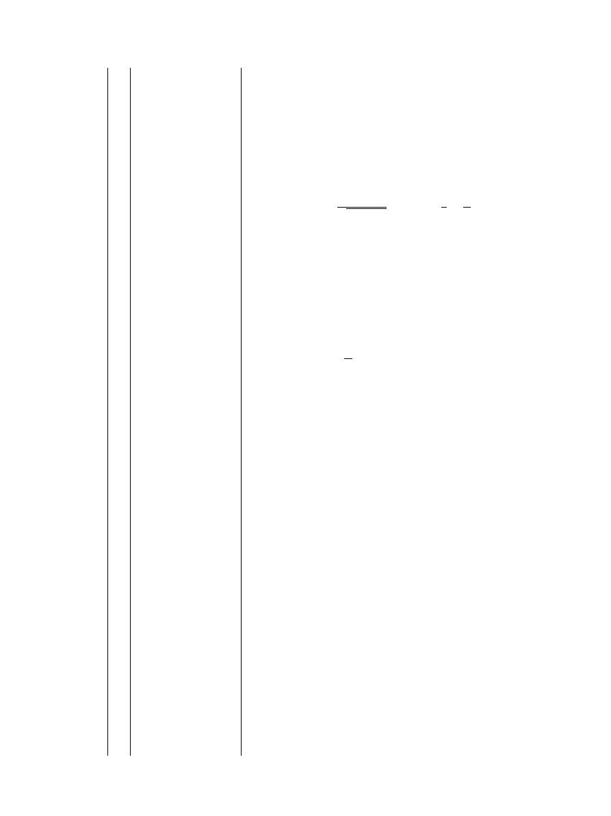
Random
forest
(RF)
is
a
bagging
algorithm
for
regression
and
classification
problems
proposed
by
Breiman
(2001)
.
This
is
a
low-
variance
method,
which
randomly
split
the
training
data
and
the
input
variables
predictors
to
build
a
set
of
b
decision
trees
(
B
t
).
The
results
of
all
decision
trees
generated
from
bootstrapped
train-
ing
samples
(
T
b
(
x
;
b
)
)
are
then
averaged,
i.e.
the
final
result
(
ˆ
y
(
x
)
)
is
the
average
of
the
output
of
all
decision
trees
(as
shown
in
Eq.
(3)
).
This
procedure
ensures
the
reduction
of
the
model
vari-
ance
and
consequently
the
reduction
of
the
risk
of
overfitting.
A
simplified
conceptual
diagram
of
the
RF
method
is
shown
in
Fig.
1
.
ˆ
y
(
x
)
=
1
B
t
B
t
b
=1
T
(
x
;
b
)
(3)
In
this
paper,
the
R
package
‘RandomForest’
(
Liaw
and
Wiener,
2002
)
was
used
for
constructing
both
non-deposition,
without
deposited
bed
and
deposited
bed,
self-cleansing
models.
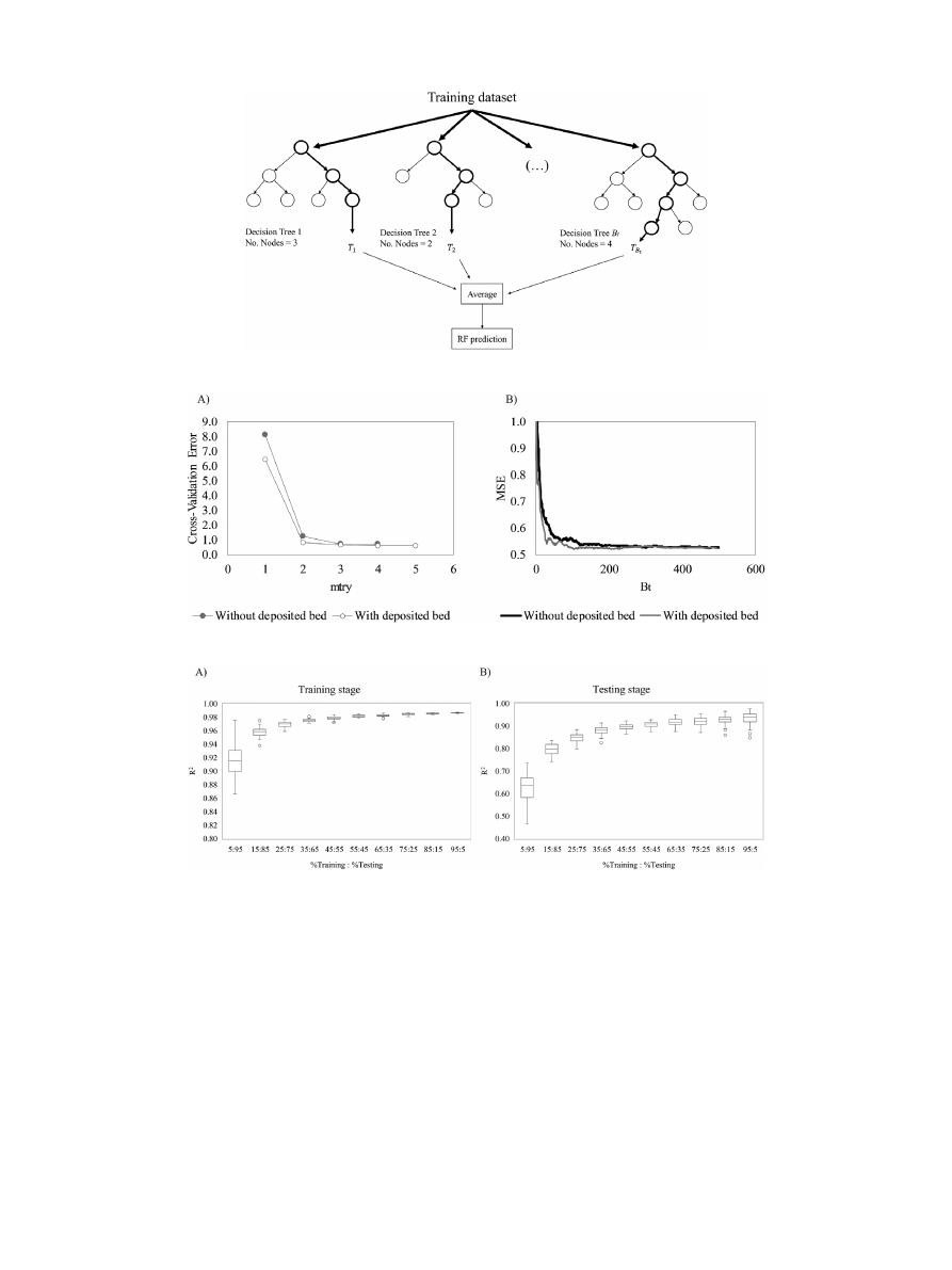
The
number
of
predictors
considered
at
each
split
(
mtry
)
and
the
number
of
trees
in
the
forest
(
B
t
)
are
the
parameters
that
define
the
structure
of
the
RF
regression
model.
The
mtry
parameter
is
estimated
by
using
the
rfcv()
function,
which
shows
the
cross-
validation
performance
for
each
number
of
predictors.
In
addition,
the
optimal
number
of
trees
is
defined
as
the
value
that
minimises
the
Mean
Square
Error
(MSE)
value
of
the
training
data.
These
pa-
rameters
are
estimated
and
the
results
are
shown
in
Fig.
2
.
Accord-
ing
to
this
figure,
the
optimal
number
of
features
(i.e.
the
random
predictors
used
in
each
tree)
are
three
and
four
non-dimensional
parameters
for
the
cases
of
without
deposited
bed
and
with
de-
posited
bed,
respectively.
Similarly,
the
optimal
number
of
trees
is
471
for
without
deposited
bed
and
229
for
with
deposited
bed.
Cross-validation
is
carried
out
during
the
training
stage
using
out-of-bag
(OOB)
samples.
As
mentioned
above,
the
method
ran-
domly
bootstraps
the
training
sample,
that
is,
some
of
the
train-
ing
data
are
left
out
to
build
each
decision
tree.
Only
two
out
of
three
parts
of
the
total
training
data
are
used
to
build
the
tree
(
Breiman,
2001
).
Based
on
this,
data
not
included
in
the
boot-
strapped
sample
(OOB
data)
are
predicted,
and
the
prediction
error
is
averaged
over
the
trees
that
do
not
include
these
data
(OOB
Er-
ror).
3.1.1.
Splitting
of
training
and
testing
data
The
whole
benchmarking
data
collected
from
the
literature
are
used
for
both
training
and
testing
stages
of
the
RF
model.
Usually,
75%
of
the
data
is
used
during
the
training
stage
of
the
model
and
the
other
25%
to
validate
the
results.
According
to
Safari
(2020)
,
the
range
of
variation
in
the
training
data
has
direct
implications
for
model
performance
(i.e.
accuracy).
As
a
result,
the
model
can
show
overfitting
issues
and
poor
extrapolation
capabilities
when
narrow
datasets
are
used
in
the
training
stage
(i.e.
data
with
a
low
range
of
variation).
3
C.
Montes, Z. Kapelan and J. Saldarriaga
Water
Research 189 (2021) 116639
Fig.
1. Simplified conceptual diagram of the RF method.
Fig.
2. Selection of the optimal Random forest parameters.
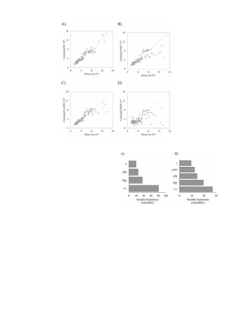
Fig.
3. Variation of the training and testing error using different combination of percentages between the training and testing dataset. A) Training stage and B) Testing stage.
Checking
the
non-overfitting
of
the
RF
model
is
carried
out
by
using
several
sizes
in
the
training
and
testing
data
(i.e.
changing
the
percentage
of
data
used
as
training
and
testing)
and
by
ver-
ifying
the
error,
defined
by
the
Coefficient
of
Determination
(
R
2
)
(as
shown
in
Eq.
(14)
).
For
this,
ten
different
combinations
of
per-
centages
are
defined
(i.e.
%
of
the
training
data
:
%
of
the
test-
ing
data
=
[5:95,
15:85,
25:75,
35:65,
45:55,
55:45,
65:35,
75:25,
85:15,
95:5]),
randomly
changing
the
ranges
of
the
training
and
testing
data,
and
developing
100
RF
models
for
each
combination.
As
a
result,
10
0
0
RF
models
are
trained
and
the
error
is
estimated
for
both
training
and
testing
stage.
Using
this
information,
several
boxplots
are
constructed
showing
the
R
2
variation
for
each
stage.
Fig.
3
shows
how
the
model
error
decreases
as
the
training
sam-
ple
size
increases.
For
example,
when
only
5%
of
the
whole
dataset
is
used
for
training
the
model
and
the
remaining
95%
for
testing
it,
the
error
varies
between
0.84
and
0.96,
for
the
training
stage,
and
between
0.39
and
0.73
for
the
testing
stage.
This
clearly
shows
that
the
model
is
under-trained;
however,
when
the
ratio
is
greater
than
50:50
the
error
tends
to
be
constant
and
slightly
variable
for
both
stages.
Ratios
greater
than
90:10
tend
to
generate
unsatis-
factory
results
for
the
testing
stage,
i.e.
the
model
is
over-trained
and
shows
high
variation
in
the
error,
i.e.
overfitting,
(as
shown
in
Fig.
3
b).
Based
on
this,
a
combination
of
75:25
is
taken
as
optimal
for
implementing
the
model.
The
variation
of
the
data
used
for
training
and
testing
dataset
is
presented
in
Table
2
.
Using
the
above
considerations,
the
RF
model
is
implemented
with
the
optimal
parameters
defined
in
Fig.
2
and
using
the
ranges
of
variation
of
the
training
data
outlined
in
Table
2
.
The
full
data
collected
from
the
literature
are
shown
in
the
Supplementary
ma-
terial.
Table
S1
and
Table
S2
show
the
data
for
non-deposition
without
and
with
deposited
bed,
respectively,
and
the
correspond-
4
C.
Montes, Z. Kapelan and J. Saldarriaga
Water
Research 189 (2021) 116639
Table
2
Variation
of the data for training and testing the RF model.
Non-deposition
criterion
Stage
No.
of runs
Channel
geometry
(mm)
Flow
Velocity (m/s)
Pipe
slope (%)
Sediment
Concentration
(ppm)
Sediment
thickness
bed
(mm)
Without
deposited bed
Training
498
D
= 100.0 – 595.0
W
= 311.5 – 462.3
0.237
- 1.41
0.04
– 3.43
0.53
– 19,957
–
Testing
166
D
= 100.0 – 595.0
W
= 311.5 – 462.3
0.237
– 1.24
0.04
– 2.74
1.00
– 13,840
–
With
deposited bed
Training
340
D
= 225 – 595
0.294
– 1.53
0.05
– 5.42
3.50
- 10,274
0.78
– 129.6
Testing
114
D
= 225 – 595
0.319
– 1.28
0.05
– 2.58
17.00
- 9101
1.78
– 120.0
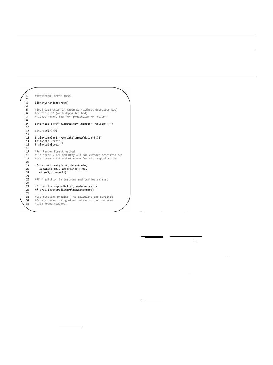
Fig.
4. Random Forest code to calculate the particle Froude number in sewer pipes.
.
ing
RF
particle
Froude
number
predictions.
The
implemented
code
for
the
RF
method
is
shown
in
Fig.
4
.
An
example
of
one
of
the
471
decision
trees
generated
by
the
RF
model,
for
the
non-deposition
without
deposited
bed,
is
shown
in
Figure
S1,
in
the
Supplemen-
tary
material.
3.1.2.
Measure
of
feature
importance
Note
that
in
this
paper,
a
decrease
in
model
accuracy
when
the
j
th
variable
is
permuted
(i.e.
the
percentage
of
the
increase
in
the
MSE,
%
IncMSE)
is
considered
as
a
measure
of
the
importance
of
a
model
input
variable.
This
index
shows
the
strength
of
each
ex-
planatory
variable
based
on
the
reduction
of
the
MSE.
The
step-
by-step
to
calculate
the
%
IncMSE is
shown
as
follows
(
Hastie
et
al.,
2009
):
(1)
Calculate
the
MSE
of
the
OOB-sample
data
in
each
tree
of
the
forest
(
MS
E
b
).
(2)
Randomly
permute
the
value
of
the
j
th
explanatory
variable
and
calculate
the
MSE
(
MS
E
j
).
(3)
Finally,
calculate
%
IncMSE for
each
explanatory
variable
as:
%
IncM
SE
=
100
·
M
S
E
j
− M
S
E
b
M
S
E
b
(4)
As
a
result,
the
more
the
%
IncMSE increases
for
a
variable,
the
more
important
it
is.
3.2.
Performance
assessment
3.2.1.
Models
used
for
comparing
the
RF
results
In
order
to
evaluate
the
RF
model
performance,
it
is
com-
pared
to
several
literature
models.
The
models
selected
for
com-
parison
are
the
replicable
white-box
models
with
high
predic-
tion
accuracy
reported
in
the
literature
and
two
black-box
mod-
els
where
the
implementing
code
is
provided
in
the
original
pa-
pers.
Other
black-box
models
cannot
be
evaluated
due
to
the
lim-
ited
replicability
shown
by
these
models
(e.g.
ANN).
Based
on
this,
in
the
case
of
non-deposition
without
deposited
bed,
seven
mod-
els
selected
are
the
EPR-MOGA
model
(
Montes
et
al.,
2020a
),
the
GEP
model
(
Kargar
et
al.,
2019
),
the
MARS
model
(
Safari,
2019
),
the
May
et
al.
(1996)
model,
the
Safari
and
Aksoy
(2020)
model,
the
ANFIS-PSO
model
(
Ebtehaj
et
al.,
2019
)
and
the
ELM
model
(
Ebtehaj
et
al.,
2020
).
In
the
case
of
non-deposition
with
de-
posited
bed,
three
models
used
for
comparison
are
the
PSO
model
(
Safari
and
Shirzad,
2019
),
the
LASSO
model
(
Montes
et
al.,
2020b
)
and
the
MGP
model
(
Safari
and
Danandeh
Mehr,
2018
).
The
EPR-
MOGA,
LASSO,
May
et
al.
(1996)
and
Safari
and
Aksoy
(2020)
are
the
regression
type
models
whilst
GEP,
MARS,
ANFIS-PSO,
ELM,
PSO
and
MGP
models
make
use
of
ML/AI
techniques.
The
equations
used
by
above
ten
models
are
as
follows:
EPR-MOGA:
V
l
gd
(
S
s
− 1
)
=
5
.
6
C
0
.
16
v
d
R
−0
.
58
S
0
.
14
o
D
0
.
02
gr
(5)
GEP:
V
l
gd
(
S
s
− 1
)
=
3
.
05
C
0
.
16
v
atan
atan
d
R
+
atan
(
3
.
41
− ln
(
D
gr
)
)
+
atan
⎛
⎝
tan
8
.
37
− 7
.
99
λ
+
d
R
λ
2
2
⎞
⎠
+
ln
⎛
⎝
d
R
3
2
λ
⎞
⎠
(6)
MARS:
V
l
gd
(
S
s
− 1
)
=
7
.
26
− 1
.
75
· max
(
0
,
d
/R
− 0
.
12
)
+
2
· max
(
0
,
0
.
12
− d/R
)
+15
.
89
· max
(
0
,
C
v
− 0
.
44
)
− 16
.
42
· max
(
0
,
0
.
44
− C
v
)
+0
.
47
· max
(
0
,
D
gr
− 0
.
29
)
− 7
.
25
· max
(
0
,
λ
− 0
.
3
)
−16
.
03
· max
(
0
,
C
v
− 0
.
01
)
+
3
.
7
· max
(
0
,
D
gr
− 0
.
12
)
−4
.
33
· max
(
0
,
D
gr
− 0
.
08
)
+
0
.
43
· max
(
0
,
λ
− 0
.
59
)
+6
.
75
· max
(
0
,
λ
− 0
.
28
)
+
1
.
67
· max
(
0
,
d
/R
− 0
.
07
)
(7)
5

C.
Montes, Z. Kapelan and J. Saldarriaga
Water
Research 189 (2021) 116639
May
et
al.
(1996)
:
C
v
=
0
.
0303
D
2
A
d
D
0
.
6
1
−
V
t
V
l
4
V
l
2
gD
(
S
s
− 1
)
1
.
5
(8)
Safari
and
Aksoy
(2020)
:
V
l
gd
(
S
s
− 1
)
=
4
.
83
C
0
.
09
v
d
R
−0
.
32
D
−0
.
14
gr
P
B
0
.
20
(9)
ANFIS-PSO:
No
equation.
The
Matlab
code
can
be
found
in
Ebtehaj
et
al.
(2019)
.
ELM:
V
l
gd
(
S
s
− 1
)
=
1
(
1
+
exp
(
−InW
· InV
+
BHI
)
)
T
· OutW
(10)
where
InW
and
OutW
are
the
input
and
output
weights,
BHI the
bias
of
the
hidden
neurons
and
InV
the
input
variables
(i.e.
C
v
,
d
/R
,
D
2
/A
,
R
/D
,
D
gr
,
d
/D
and
λ
).
Full
details
of
the
values
chosen
for
each
parameter
are
shown
in
Ebtehaj
et
al.
(2020)
.
PSO:
V
l
gd
(
S
s
− 1
)
=
3
.
66
C
0
.
16
v
d
R
−0
.
40
y
s
Y
−0
.
10
(11)
LASSO:
V
l
gd
(
S
s
− 1
)
=
5
.
83
C
0
.
144
v
d
R
−0
.
305
λ
−0
.
059
D
−0
.
169
gr
y
s
D
−0
.
104
(12)
MGP:
V
l
gd
(
S
s
− 1
)
=
1
.
96
− 0
.
61
λ
− 0
.
51
C
v
+
1
.
18
D
0
.
50
gr
λ
1
.
50
+
0
.
61
2
C
v
+
d
R
0
.
50
− 2
.
45
d
R
1
/
8
(13)
3.2.2.
Performance
indices
The
RF
model
performance
is
evaluated
and
compared
to
above
ten
models
using
three
performance
indicators.
These
are
the
Co-
efficient
of
Determination
(
R
2
),
the
Root
Mean
Square
Error
(
RMSE
)
and
the
Mean
Absolute
Percentage
Error
(
MAPE
),
defined
as
fol-
lows:
R
2
=
1
−
n
i
=1
F
∗
r
OBS
− F
r
MOD
2
n
i
=1
F
∗
r
OBS
− F
∗
r
OBS
2
(14)
RMSE
=
1
n
n
i
=1
F
∗
r
OBS
− F
r
MOD
2
(15)
MAP
E
=
100
n
n
i
=1
F
∗
r
OBS
− F
r
MOD
F
∗
r
OBS
(16)
where
F
∗
r
OBS
is
the
particle
Froude
number
observed
data,
F
r
MOD
the
particle
Froude
number
estimated
by
RF
algorithm
(or
other
pre-
dictive
model),
n
the
number
of
data
and
F
∗
r
OBS
the
mean
of
ob-
served
particle
Froude
number
data.
The
Coefficient
of
Determination
measures
the
percentage
of
the
model
variance
that
can
be
explained.
This
coefficient
varies
between
0
and
1,
with
a
value
of
1
denoting
a
perfect
match
be-
tween
observed
and
modelled
data.
The
Root
Mean
Square
Error
measures
the
standard
deviation
of
the
residuals.
Note
that
a
value
close
to
0
indicates
high
model
prediction
accuracy.
Finally,
the
Mean
Absolute
Percentage
Error
assesses
the
model
prediction
ac-
curacy
(i.e.
bias)
as
a
percentage
of
the
observed
value.
Value
of
0
indicates
the
perfect
model
where
there
are
no
differences
be-
tween
predictions
and
observations.
4.
Results
The
results
obtained
by
using
the
methodology
shown
in
the
previous
section
are
presented
in
Tables
3
and
4
,
for
without
de-
posited
bed
and
deposited
bed
criteria,
respectively.
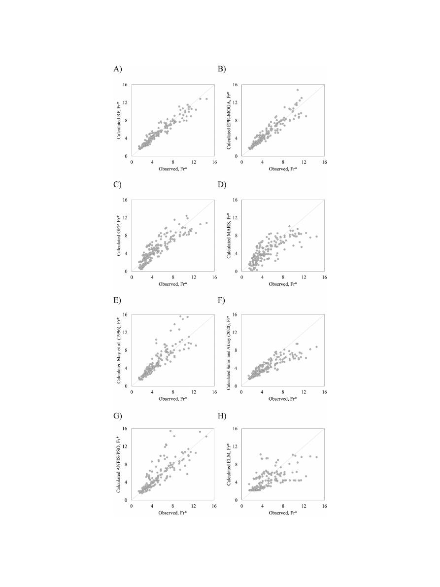
Graphically,
these
results
are
shown
in
Figs.
5
and
6
.
As
shown
in
these
tables,
for
the
MARS,
ANFIS-PSO,
ELM
and
MGP
models,
the
outliers
of
the
particle
Froude
number
(i.e.
F
r
∗
<
0.00
and
F
r
∗
>
20.00)
were
re-
moved.
This
is
because
these
models
can
produce
extreme
values
(e.g.
F
r
∗
=
−58.67
or
F
r
∗
=
163.59,
among
others)
that
misrepresent
the
model
comparison
when
evaluating
the
performance
indices.
As
it
can
be
seen
from
Table
3
,
Random
Forest
model
shows
a
better
generalisation
capacity
than
other
models
shown,
as
demonstrated
in
high
prediction
accuracy
observed
for
all
avail-
able
datasets
(0.88
>
R
2
>
0.98,
0.24
>
RMSE
>
0.73
and
4.36%
>
MAP
E
>
11.09%).
The
following
observations
can
be
made
from
the
performance
of
the
other
models
evaluated:
•
EPR-MOGA,
similarly
to
RF,
shows
good
results
but
has
infe-
rior
accuracy
in
large
sewer
pipes
(
R
2
=
0.86,
RMSE
=
1.03
and
MAP
E
=
11.31%).
In
addition,
EPR-MOGA
model
shows
limita-
tions
for
predicting
the
particle
Froude
number
in
non-circular
sections
(as
shown
in
the
Mayerle
(1988)
rectangular
data).
This
equation
shows
good
extrapolation
capabilities
because
of
the
inclusion
of
the
pipe
slope
as
input
feature
for
the
self-
cleansing
prediction.
•
GEP
shows
acceptable
results
(0.79
>
R
2
>
0.87,
0.66
>
RMSE
>
0.89
and
11.45%
>
MAP
E
>
22.33%)
for
the
datasets
used
for
its
development
in
circular
channels
(
Ab
Ghani,
1993
;
Mayerle,
1988
;
Vongvisessomjai
et
al.,
2010
)
and
poor
perfor-
mance
for
other
datasets
(0.00
>
R
2
>
0.76,
1.00
>
RMSE
>
1.95
and
14.35%
>
MAP
E
>
37.92%).
This
model
presents
good
performance
for
large
sewer
pipes.
In
contrast,
for
non-circular
channels
the
model
quickly
loss
accuracy.
•
According
to
Safari
(2019)
,
MARS
model
was
developed
by
us-
ing
the
experimental
data
collected
by
Mayerle
(1988)
(in
both
circular
and
rectangular
channels),
May
(1993)
,
Ab
Ghani
(1993)
and
Vongvisessomjai
et
al.
(2010)
.
As
a
result,
this
model
shows
acceptable
performance
for
these
datasets
(0.49
>
R
2
>
0.87,
0.81
>
RMSE
>
1.15
and
13.63%
>
MAP
E
>
28.08%)
but
poor
performance
for
the
remaining
datasets
(
R
2
=
0.00,
1.48
>
RMSE
>
2.88
and
29.14%
>
MAP
E
>
51.28%).
Based
on
the
above,
and
compared
to
the
RF
model,
limited
extrapolation
capabilities
are
identified
for
the
MARS
model.
•
May
et
al.
(1996)
is
the
best
regression-based
equation
re-
ported
in
the
literature
(
Ackers
et
al.,
2001
;
Ebtehaj
et
al.,
2014
),
as
it
was
developed
using
several
experimental
datasets.
This
is
the
equation
proposed
by
the
Construction
Industry
Re-
search
and
Information
Association
(CIRIA)
for
designing
self-
cleansing
sewer
pipes
transporting
coarser
granular
material
as
bedload
(
Ackers
et
al.,
2001
).
This
model
shows
good
perfor-
mance
for
pipe
diameters
less
than
500
mm
(0.83
>
R
2
>
0.99,
0.13
>
RMSE
>
0.82
and
2.38%
>
MAP
E
>
11.61%).
In
con-
trast,
limited
extrapolation
for
large
sewer
pipes
is
identified
as
the
low
performance
indices
values
obtained
(
R
2
=
0.00,
RMSE
=
4.88
and
MAP
E
=
48.97%).
This
equation
shows
better
performance
than
the
RF
model
when
compared
to
data
from
Vongvisessomjai
et
al.
(2010)
,
but
lower
accuracy
when
applied
to
the
rest
of
the
datasets.
6

C.
Montes, Z. Kapelan and J. Saldarriaga
Water
Research 189 (2021) 116639
Table
3
Accuracy
of self-cleansing models for without deposited bed criterion using performance indices for training and testing dataset. Bolded values show best performance
model.
Dataset
Performance
Index
Model
RF
EPR-MOGA
GEP
MARS
May
et al. (1996) a Safari and Aksoy (2020)
ANFIS-PSO
ELM
Training
R
2
0.98
0.90
0.75
0.00
0.27
0.74
0.51
∗
0.30
∗
RMSE
0.33
0.76
1.22
2.55
2.17
1.25
1.69
∗
1.95
∗
MAPE
(%)
4.88
11.54
23.52
34.16
17.49
17.21
19.32
∗
29.76
∗
Testing
R
2
0.91
0.86
0.69
0.00
0.09
0.74
0.40
∗
0.32
∗
RMSE
0.73
0.88
1.33
2.55
2.27
1.21
1.84
∗
1.92
∗
MAPE
(%)
11.09
12.35
26.43
36.57
19.15
17.24
20.95
∗
29.82
∗
Mayerle
(1988)
circular
R
2
0.96
0.89
0.87
0.87
0.87
0.75
0.80
∗
0.42
RMSE
0.45
0.75
0.81
0.81
0.82
1.12
1.00
∗
1.71
MAPE
(%)
5.62
8.90
14.77
14.03
11.49
14.91
17.92
∗
26.75
Mayerle
(1988)
rectangular
R
2
0.93
0.38
0.30
0.81
–
0.87
0.00
0.47
RMSE
0.49
1.44
1.54
0.81
–
0.66
2.74
1.33
MAPE
(%)
8.49
28.97
33.00
15.51
–
13.14
45.28
20.75
Ab
Ghani (1993)
R
2
0.97
0.96
0.83
0.72
0.90
0.81
0.88
0.38
RMSE
0.36
0.43
0.89
1.15
0.67
0.94
0.74
1.69
MAPE
(%)
5.94
9.35
22.33
28.08
10.32
15.60
10.34
23.96
Ota
(1999)
R
2
0.97
0.98
0.44
0.00
0.96
0.97
0.97
0.55
RMSE
0.24
0.20
1.00
1.48
0.27
0.25
0.22
0.90
MAPE
(%)
5.55
6.90
37.92
51.28
7.78
7.90
6.46
19.54
Vongvisessomjai
et al. (2010)
R
2
0.88
0.95
0.79
0.49
0.99
0.71
0.97
0.00
RMSE
0.49
0.33
0.66
1.03
0.13
0.78
0.24
1.59
MAPE
(%)
6.56
5.78
11.45
13.63
2.38
13.34
3.62
28.50
Montes
et al. (2020a)
R
2
0.96
0.98
0.00
0.00
0.83
0.67
0.77
∗
0.00
RMSE
0.31
0.25
1.64
2.37
0.67
0.94
0.75
∗
1.85
MAPE
(%)
4.36
4.94
28.15
49.73
11.61
15.39
12.39
∗
33.96
Montes
et al. (2020b)
R
2
0.94
0.86
0.76
0.00
∗
0.00
0.34
0.00
∗
0.00
∗
RMSE
0.70
1.03
1.37
2.88
∗
4.88
2.26
3.01
∗
3.10
∗
MAPE
(%)
7.33
11.31
14.35
29.14
∗
48.97
23.44
30.56
∗
39.30
∗
a
Model not valid for non-circular channels.
∗
Outliers
removed.
Table
4
Accuracy
of self-cleansing models for deposited bed criterion using performance in-
dices
for training and testing dataset. Bolded values show best performance model.
Dataset
Performance
Index
Model
RF
PSO
LASSO
MGP
Training
R
2
0.98
0.75
0.82
0.51
∗
RMSE
0.32
1.30
1.13
1.69
∗
MAPE
(%)
4.70
14.36
13.07
28.78
∗
Testing
R
2
0.91
0.70
0.83
0.29
∗
RMSE
0.80
1.47
1.10
2.19
∗
MAPE
(%)
12.10
15.94
12.59
31.36
∗
El-Zaemey
(1991)
R
2
0.94
0.78
0.83
0.54
RMSE
0.38
0.76
0.66
1.08
MAPE
(%)
6.49
14.28
11.97
30.19
Perrusquía
(1991)
R
2
0.84
0.65
0.62
0.00
RMSE
0.33
0.49
0.50
1.29
MAPE
(%)
7.07
10.15
12.05
30.58
Ab
Ghani (1993)
R
2
0.91
0.56
0.74
0.51
RMSE
0.60
1.32
1.01
1.40
MAPE
(%)
6.13
16.26
11.19
13.07
May
(1993)
R
2
0.90
0.63
0.64
0.54
RMSE
0.62
1.18
1.16
1.31
MAPE
(%)
6.50
13.47
14.26
14.21
Montes
et al. (2020a)
R
2
0.93
0.00
0.73
0.00
∗
RMSE
0.81
3.06
1.56
5.54
∗
MAPE
(%)
6.84
21.05
10.36
58.79
∗
∗
Outliers
removed.
•
Safari
and
Aksoy
(2020)
model
is
a
competitive
equation
for
predicting
the
self-cleansing
velocity
in
both
circular
and
non-
circular
channels.
This
model
shows
similar
but
inferior
per-
formance
to
EPR-MOGA
model
in
small
sewer
pipes
(0.67
>
R
2
>
0.97,
0.25
>
RMSE
>
1.12
and
7.90%
>
MAP
E
>
15.60%),
but
in
large
sewers
the
accuracy
is
quickly
lost
(
R
2
=
0.34,
RMSE
=
2.26
and
MAP
E
=
23.46%).
In
contrast,
this
model
outperforms
the
results,
compared
to
other
regression
models
(EPR-MOGA,
GEP
and
MARS)
and
ML/AI
models
(ANFIS-PSO
and
ELM),
in
non-circular
channels
(
R
2
=
0.87,
RMSE
=
0.66
and
MAP
E
=
13.41%),
which
is
a
competitive
performance
compared
to
the
RF
model
(
R
2
=
0.89,
RMSE
=
0.61
and
MAP
E
=
10.05%).
This
is
because
of
the
inclusion
of
the
P
/B
relation
as
explana-
tory
variable
for
predicting
the
particle
Froude
number.
This
model
is
competitive
and
shows
good
generalisation
of
the
problem
for
designing
sewers
under
the
non-deposition
with-
out
deposited
bed
criterion.
•
According
to
Ebtehaj
et
al.
(2019)
,
ANFIS-PSO
model
was
developed
by
using
the
experimental
data
collected
by
Ab
Ghani
(1993)
,
Ota
(1999)
and
Vongvisessomjai
et
al.
(2010)
.
As
a
result,
this
model
shows
good
performance
for
these
datasets
(0.88
>
R
2
>
0.97,
0.22
>
RMSE
>
0.74
and
3.62%
>
MAP
E
>
10.34%).
In
large
sewers
and
non-circular
channels,
the
model
losses
accuracy
(
R
2
=
0.00,
2.74
>
RMSE
>
3.01
and
30.56%
>
MAP
E
>
45.28%).
This
model
produces
some
extreme
values
when
the
particle
Froude
number
is
calculated,
espe-
cially
in
the
Montes
et
al.
(2020b)
dataset.
The
RF
model
gen-
erates
better
results
compared
to
this
model.
•
ELM
was
trained
with
the
same
dataset
used
for
the
ANFIS-PSO
model.
Not
satisfactory
results
are
obtained
when
this
model
is
applied
on
the
dataset
considered
in
this
study
(0.00
>
R
2
>
0.55,
0.90
>
RMSE
>
3.1
and
19.54%
>
MAP
E
>
39.30%).
Same
comments,
as
mentioned
above
for
the
ANFIS-PSO
model,
can
be
shown
here.
According
to
the
results
shown
in
Table
4
(deposited
bed
crite-
rion),
RF
model
outperforms
the
other
models
for
the
entire
con-
sidered
dataset.
This
model
shows
good
accuracy
levels
(0.84
>
R
2
>
0.98,
0.32
>
RMSE
>
0.81
and
4.70%
>
MAP
E
>
12.10%)
for
all
the
range
of
variation
of
the
hydraulics
and
sediment
characteris-
tics.
Comments
related
to
the
other
models
studied
are
as
follows:
7
C.
Montes, Z. Kapelan and J. Saldarriaga
Water
Research 189 (2021) 116639
Fig.
5. Performance of the models applied in the non-deposition without deposited bed testing dataset.
8
C.
Montes, Z. Kapelan and J. Saldarriaga
Water
Research 189 (2021) 116639
Fig.
6. Performance of the models applied in the non-deposition with deposited bed testing dataset. .
•
PSO
model
was
developed
by
using
the
experimental
data
col-
lected
by
El-Zaemey
(1991)
,
Perrusquía
(1991)
,
May
(1993)
and
Ab
Ghani
(1993)
.
As
a
result,
this
model
shows
good
perfor-
mance
for
these
datasets
(0.56
>
R
2
>
0.78,
0.49
>
RMSE
>
1.32
and
10.15%
>
MAP
E
>
16.26%).
However,
when
the
model
is
compared
to
the
data
collected
in
the
large
sewer
pipe,
the
accuracy
quickly
decreases
(
R
2
=
0.00,
RMSE
=
3.06
and
MAP
E
=
21.05%).
•
LASSO
model
reports
good
accuracy
levels
for
all
the
datasets
considered
(0.62
>
R
2
>
0.83,
0.50
>
RMSE
>
1.56
and
10.36%
>
MAP
E
>
14.26%).
However,
the
accuracy
is
still
inferior
com-
pared
to
the
RF
model.
This
model
shows
good
extrapolation
capabilities
and
generalisation
of
the
problem.
•
MGP
was
developed
by
using
the
same
experimental
datasets
of
the
PSO
model.
This
model
shows
less
accuracy
compared
to
the
PSO
model
(0.00
>
R
2
>
0.54,
1.08
>
RMSE
>
5.54
and
13.07%
>
MAP
E
>
58.79%).
In
large
sewer
pipes,
the
model
shows
poor
performance.
In
contrast
to
other
models,
the
MGP
was
developed
by
using
normalised
values.
Based
on
this,
the
range
of
variation
used
for
training
the
model
can
potentially
affect
the
final
form/structure
of
the
final
expression
shown
by
the
MGP.
RF
accuracy
shown
in
the
Montes
et
al.
(2020b)
data
is
es-
pecially
important
due
to
the
relative
sediment
thickness
(
y
s
/D
)
used
at
laboratory
scale
in
that
study.
As
Table
1
shows,
the
sedi-
ment
thickness
used
at
laboratory
scale
ranging
from
0.8
mm
(for
Montes
et
al.
(2020b)
data)
to
129.6
mm
(for
May
(1993)
data),
i.e.
the
variation
of
y
s
/D
is
from
1.1%
to
20.0%
of
the
pipe
diame-
ter.
Values
of
y
s
/D
=
20%
is
an
unrealistic
consideration
since
the
optimal
sediment
thickness
design
has
been
defined
as
1%
of
the
pipe
diameter
(
May
et
al.,
1989
;
Safari
and
Shirzad,
2019
).
Data
collected
by
Montes
et
al.
(2020b)
seem
to
be
the
closer
repre-
sentation
of
the
real
conditions
found
in
sewer
systems.
Based
on
Fig.
7. Variable importance estimated by RF model: A) without deposited bed; B)
with
deposited bed.
this,
RF
is
the
model
that
best
predicts
the
self-cleansing
velocity
for
data
close
to
real
conditions.
4.1.
Variable
importance
RF
model
input
variable
importance
is
presented
in
Fig.
7
.
As
shown
in
this
figure,
for
both
non-deposition
criteria
the
most
important
variable
is
the
volumetric
sediment
concentration,
fol-
lowed
by
the
dimensionless
grain
size
and
the
relative
grain
size.
This
result
is
consistent
with
previous
findings
reported
in
the
lit-
erature
(
Ackers
et
al.,
2001
;
Ebtehaj
et
al.,
2020
).
Less
important
parameters
for
predicting
the
particle
Froude
number
and
thus
the
self-cleansing
velocity,
are
the
relative
sediment
thickness
and
the
channel
friction
factor,
for
the
deposited
bed
criterion.
Parameter
importance
shown
by
EPR-MOGA,
Safari
and
Ak-
soy
(2020)
,
PSO
and
LASSO
is
quite
different.
In
these
tech-
niques,
the
most
important
parameter
is
the
relative
grain
9

C.
Montes, Z. Kapelan and J. Saldarriaga
Water
Research 189 (2021) 116639
size
due
to
the
highest
values
of
the
regression
coefficients
(
(
d
R
)
−c
; 0
.
305
<
c
<
0
.
58
)
,
as
shown
in
Eqs.
(5)
,
(9)
,
(11)
and
(12)
.
The
parameter
importance
for
the
GEP,
MARS
and
MGP
model
is
less
intuitive
because
of
the
form
of
the
equations,
as
shown
in
Eqs.
(6)
,
(7)
and
(13)
,
which
include
logarithmic
and
inverse
tangent
functions
for
calculating
the
particle
Froude
number.
Less
comparable
are
the
results
shown
by
ANFIS-PSO
and
ELM
since
no
practical
equation
is
provided.
Based
on
the
above
results
shown
in
Fig.
7
,
a
good
estimate
of
the
volumetric
sediment
concentration
seems
to
be
essential
for
increasing
the
accuracy
of
the
calculation
of
the
particle
Froude
number
and
consequently
the
minimum
self-cleansing
velocity
for
both
non-deposition
criteria.
In
addition,
hydraulic
characteristics
of
the
pipe
(defined
by
the
hydraulic
radius)
and
the
sediment
characteristics
(i.e.
particle
diameter
and
specific
gravity)
are
pro-
portionally
important
for
model
performance.
5.
Discussion
The
prediction
of
self-cleansing
conditions
in
sewers
remains
a
challenge
despite
multiple
models
and
equations
developed
and
reported
in
the
literature.
Existing
regression-based
equations
and
AI/ML
models
show
limited
generalisation
capabilities
and
overfit-
ting
problems.
In
this
paper,
a
new
approach
for
addressing
these
issues
is
proposed
by
using
the
Random
Forest
method.
Due
to
the
nature
of
the
RF
method,
where
the
model
variance
is
reduced
by
averaging
the
results
from
an
ensemble
of
decision
trees,
the
risk
of
overfitting
is
low.
By
using
a
reduced
number
of
input
features
for
constructing
each
decision
tree
in
the
forest,
the
correlation
between
base
trees
is
avoided.
This
is
an
improvement
of
the
method
compared
to
a
single
decision
tree,
which
can
be
overtrained
(i.e.
the
tree
learns
the
noise
from
the
training
data)
and
thus
shows
poor
performance
in
the
testing
dataset.
RF
model
showed
good
generalisation
capabilities
when
the
whole
dataset
is
divided
into
75%
for
the
training
stage
and
25%
for
the
testing
stage.
For
this
percentage
of
split
data,
the
testing
error
presented
a
low
variance.
In
contrast,
by
increasing
the
num-
ber
of
data
used
in
the
training
stage
(e.g.
95%
of
the
whole
data)
the
testing
error
showed
high
variance,
which
is
an
indicator
of
an
over-trained
model
with
limited
extrapolation
capabilities
(as
shown
in
Fig.
3
b).
Therefore,
choosing
the
right
percentage
split
is
critical
to
avoid
model
overfitting.
Variable
importance
analysis
showed
that
the
volumetric
sedi-
ment
concentration
is
the
most
relevant
feature
for
predicting
the
self-cleansing
velocity
in
practice
for
both
non-deposition
criteria,
followed
by
the
dimensionless
grain
size.
The
self-cleansing
predic-
tion
is
no
conditioned
by
the
channel
material,
as
the
low
variable
importance
shown
by
the
channel
friction
factor.
RF
results
are
compared
to
existing
models
reported
in
the
lit-
erature
and
showed
better
performance
for
the
whole
dataset
for
both
non-deposition
without
and
with
deposited
bed
criteria.
This
is
explained
by
several
factors,
such
as:
•
RF
is
able
to
better
capture
the
non-linearity
in
the
data
com-
pared
to
linear
regression
models
(i.e.
regression-based
models
proposed
by
May
et
al.
(1996)
and
Safari
and
Aksory
(2020)
).
The
RF
model
also
better
captures
complex
interactions
be-
tween
features.
This
is
because
of
RF
model’s
ability
to
capture
effectively
non-linear
patterns
in
data.
•
RF
showed
a
good
bias-variance
trade-off (i.e.
low
bias
and
low
variance)
for
both
non-deposition
criteria.
In
contrast,
exist-
ing
non-regression
models
reported
in
the
literature
(i.e.
MARS,
ANFIS-PSO
and
ELM),
and
compared
to
the
RF
model
in
this
paper,
in
some
cases
presented
low
bias
and
high
variance
(i.e.
overfitting)
for
the
non-deposition
without
deposited
bed
crite-
rion,
as
shown
in
Fig.
5
.
For
the
non-deposition
with
deposited
bed
criterion,
the
existing
models
(i.e.
PSO,
LASSO
and
MGP)
showed
high
bias,
since
these
models
systematically
underes-
timate
the
particle
Froude
number
in
the
testing
dataset
(as
shown
in
Fig.
6
).
•
The
range
of
variation
used
for
training
and
testing
the
RF
model
is
much
larger
than
the
dataset
used
in
the
literature
for
developing
the
existing
predictive
models.
For
example,
the
ANFIS-PSO
and
ELM
were
trained
and
testing
with
the
Ab
Ghani
(1993)
,
Ota
(1999)
and
Vongvisessomjai
et
al.
(2010)
data
(i.e.
290
data
approx.).
Given
this,
the
RF
model
developed
here
is
able
to
predict
the
particle
Froude
number
for
a
larger
range
of
variation
of
the
input
conditions.
An
example
of
this
is
shown
in
Fig.
6
where
the
existing
models
reported
for
the
non-deposition
with
deposited
bed
criterion
underestimate
the
particle
Froude
number
for
values
above
9.0
(
F
r
∗
>
9.0).
Despite
the
RF
presented
in
this
study
outperforms
the
existing
models
reported
in
the
literature,
further
tests
with
data
collected
in
real
sewers
should
be
conducted.
The
cohesive
effects
of
the
de-
posited
material
must
be
included
for
future
developments.
Finally,
further
evaluation
of
the
performance
of
the
model
in
trapezoidal,
ovoid,
or
U-shape
channels
should
be
carried
out
to
check
the
ap-
plicability
of
the
model
under
these
channel
characteristics.
6.
Conclusions
Random
Forest
based
model
was
developed
for
predicting
the
self-cleansing
velocity
under
the
concept
of
non-deposition.
This
model
was
implemented
using
the
experimental
benchmark
data
reported
in
the
literature.
The
RF
model
was
compared
to
the
fol-
lowing
ten
literature
models:
EPR-MOGA,
MARS,
MGP,
ANFIS-PSO,
ELM,
LASSO,
GEP
and
PSO,
and
two
regression-based
equations
proposed
by
May
et
al.
(1996)
and
Safari
and
Aksoy
(2020)
.
The
following
conclusions
are
made
based
on
the
results
ob-
tained:
(1)
Random
Forest
model
is
able
to
predict
the
particle
Froude
number
(i.e.
minimum
self-cleansing
velocity)
for
the
non-
deposition
self-cleansing
design
criteria
with
high
accuracy
on
validation
(i.e.
unseen)
data.
This
is
due
to
the
ability
of
RF
to
better
generalise
the
analysed
data,
i.e.
the
ability
to
avoid
model
overfitting.
(2)
RF
model
prediction
accuracy
is
consistently
superior
to
ten
other
literature
models
considered
here.
This
is
likely
due
to
the
reason
mentioned
above
but
also
the
capability
to
bet-
ter
capture
the
complex
interactions
between
input
variables
when
compared
to
other
models
considered
in
this
paper.
This
is
especially
relevant
for
the
non-deposition
with
de-
posited
bed
case
where
the
accuracy
of
RF
model
predictions
is
substantially
higher
than
in
other
models
(i.e.
LASSO,
MGP
and
PSO
models).
(3)
The
volumetric
sediment
concentration
is
the
most
impor-
tant
input
variable
for
predicting
the
self-cleansing
veloc-
ity
in
sewer
pipes.
A
good
characterisation
of
this
parame-
ter
seems
to
be
essential
for
improving
the
design
of
new
self-cleansing
sewers.
Based
on
the
above,
RF
can
be
used
for
predicting
self-cleansing
velocity
with
high
accuracy,
especially
for
large
sewer
pipes
with
the
presence
of
deposited
bed.
This
technique
can
be
used
for
de-
signing
self-cleansing
sewer
systems.
Further
testing
of
the
RF
and
other
self-cleansing
models
in
real
sewer
systems
is
required
to
further
validate
these
models
in
those
circumstances
and
ensure
their
applicability
in
engineering
prac-
tice.
10

C.
Montes, Z. Kapelan and J. Saldarriaga
Water
Research 189 (2021) 116639
Declaration
of
Competing
Interest
The
authors
declare
that
they
have
no
known
competing
finan-
cial
interests
or
personal
relationships
that
could
have
appeared
to
influence
the
work
reported
in
this
paper.
Funding
This
research
did
not
receive
any
specific
grant
from
funding
agencies
in
the
public,
commercial,
or
not-for-profit
sectors.
Supplementary
materials
Supplementary
material
associated
with
this
article
can
be
found,
in
the
online
version,
at
doi:
10.1016/j.watres.2020.116639
.
References
Ab
Ghani, A. , 1993. Sediment transport in sewers. PhD thesis. University of Newcas-
tle
Upon Tyne, Newcastle Upon Tyne, UK .
Ackers,
J., Butler, D., Leggett, D., May, R., 2001. Designing sewers to control sediment
problems.
In: Urban Drainage Modeling. ASCE, Orlando, FL, pp. 818–823. doi:
10.
1061/40583(275)77
.
Breiman,
L., 2001. Random forests. Mach. Learn. 45, 5–32. doi:
10.1023/A:
1010933404324
.
Ebtehaj,
I., Bonakdari, H., 2016a. Bed load sediment transport in sewers at limit of
deposition.
Sci. Iran. 23 (3), 907–917. doi:
10.24200/sci.2016.2169
.
Ebtehaj,
I., Bonakdari, H., 2016b. A support vector regression-firefly algorithm-based
model
for limiting velocity prediction in sewer pipes. Water Sci. Technol. 73 (9),
2244–2250.
doi:
10.2166/wst.2016.064
.
Ebtehaj,
I., Bonakdari, H., 2013. Evaluation of sediment transport in sewer us-
ing
artificial neural network. Eng. Appl. Comput. Fluid Mech. 7 (3), 382–392.
doi:
10.1080/19942060.2013.11015479
.
Ebtehaj,
I., Bonakdari, H., Es-Haghi, M., 2019. Design of a hybrid ANFIS–PSO model
to
estimate sediment transport in open channels. Iran. J. Sci. Technol. Trans. 44
(4),
851–857. doi:
10.1007/s40996-
018- 0218- 9
.
Ebtehaj,
I., Bonakdari, H., Safari, M., Gharabaghi, B., Zaji, A., Riahi Madavar, H., Sheikh
Khozani,
Z., Es-haghi, M., Shishegaran, A., Danandeh Mehr, A., 2020. Combina-
tion
of sensitivity and uncertainty analyses for sediment transport modeling in
sewer
pipes. Int. J. Sediment Res. 35 (2), 157–170. doi:
10.1016/j.ijsrc.2019.08.005
.
Ebtehaj,
I., Bonakdari, H., Sharifi, A., 2014. Design criteria for sediment transport in
sewers
based on self-cleansing concept. J. Zhejiang Univ. Sci. A 15 (11), 914–924.
doi:
10.1631/jzus.a1300135
.
El-Zaemey,
A. , 1991. Sediment transport over deposited beds in sewers. PhD thesis.
University
of Newcastle Upon Tyne, Newcastle Upon Tyne, UK .
Hastie,
T., Tibshirani, R., Friedman, J., 2009. The elements of statistical learning:
data
mining, inference, and prediction. Springer, New York, USA doi:
10.1007/
978-
0- 387- 84858- 7
.
Kargar,
K., Safari, M., Mohammadi, M., Samadianfard, S., 2019. Sediment transport
modeling
in open channels using neuro-fuzzy and gene expression program-
ming
techniques. Water Sci. Technol. 79 (12), 2318–2327. doi:
10.2166/wst.2019.
229
.
Liaw,
A. , Wiener, M. , 2002. Classification and regression by Random forest. R News
2
(3), 18–22 .
May,
R. , 1993. Sediment transport in pipes and sewers with deposited beds. HR
Wallingford,
Oxfordshire, UK Report SR 320 .
May,
R., Ackers, J., Butler, D., John, S., 1996. Development of design methodol-
ogy
for self-cleansing sewers. Water Sci. Technol. 33 (9), 195–205. doi:
10.1016/
0273-
1223(96)00387- 3
.
May,
R. , Brown, P. , Hare, G. , Jones, K. , 1989. Self-cleansing conditions for sewers
carrying
sediment. HR Wallingford, Oxfordshire, UK Report SR 221 .
Mayerle,
R. , 1988. Sediment transport in rigid boundary channels. PhD thesis. Uni-
versity
of Newcastle upon Tyne, Newcastle Upon Tyne, UK .
Merritt,
L. , Enfinger, K. , 2019. Tractive force: a key to solids transport in gravity flow
drainage
pipes. In: Pipelines 2019. ASCE, Nashville, TN, pp. 349–358 .
Montes,
C., Berardi, L., Kapelan, Z., Saldarriaga, J., 2020a. Predicting bedload sed-
iment
transport of non-cohesive material in sewer pipes using evolutionary
polynomial
regression – multi-objective genetic algorithm strategy. Urban Wa-
ter
J. 17 (2), 154–162. doi:
10.1080/1573062X.2020.1748210
.
Montes,
C., Kapelan, Z., Saldarriaga, J., 2019. Impact of self-cleansing criteria choice
on
the optimal design of sewer networks in South America. Water (Basel) 11,
1148.
doi:
10.3390/w11061148
.
Montes,
C., Vanegas, S., Kapelan, Z., Berardi, L., Saldarriaga, J., 2020b. Non-deposition
self-cleansing
models for large sewer pipes. Water Sci. Technol. 81 (3), 606–621.
doi:
10.2166/wst.2020.154
.
Nalluri,
C., Ab Ghani, A., 1996. Design options for self-cleansing storm sewers. Water
Sci.
Technol. 33 (9), 215–220. doi:
10.1016/0273-
1223(96)00389- 7
.
Ota,
J. , 1999. Effect of particle size and gradation on sediment transport in storm
sewers.
PhD thesis. University of Newcastle upon Tyne, Newcastle Upon Tyne,
UK
.
Perrusquía,
G. , 1991. Bedload Transport in Storm Sewers: Stream Traction in Pipe
Channels
PhD thesis. Chalmers University of Technology, Gothenburg, Sweden .
Roushangar,
K., Ghasempour, R., 2017. Estimation of bedload discharge in sewer
pipes
with different boundary conditions using an evolutionary algorithm. Int.
J.
Sediment Res. 32 (4), 564–574. doi:
10.1016/j.ijsrc.2017.05.007
.
Safari,
M., 2019. Decision tree (DT), generalized regression neural network (GR) and
multivariate
adaptive regression splines (MARS) models for sediment transport
in
sewer pipes. Water Sci. Technol. 79 (6), 1113–1122. doi:
10.2166/wst.2019.106
.
Safari,
M., Danandeh Mehr, A., 2018. Multigene genetic programming for sediment
transport
modeling in sewers for conditions of non-deposition with a bed de-
posit.
Int. J. Sediment Res. 33 (3), 262–270. doi:
10.1016/j.ijsrc.2018.04.007
.
Safari,
M., Mohammadi, M., Ab Ghani, A., 2018. Experimental studies of self-
cleansing
drainage system design: a review. J. Pipeline Syst. Eng. Pract. 9 (4),
04018017.
doi:
10.1061/(ASCE)PS.1949-1204.0
0 0 0335
.
Safari,
M., Shirzad, A., 2019. Self-cleansing design of sewers: definition of the opti-
mum
deposited bed thickness. Water Environ. Res. 91 (5), 407–416. doi:
10.1002/
wer.1037
.
Safari,
M., Shirzad, A., Mohammadi, M., 2017. Sediment transport modeling in de-
posited
bed sewers: unified form of May’s equations using the particle swarm
optimization
algorithm. Water Sci. Technol. 76 (4), 992–10 0 0. doi:
10.2166/wst.
2017.267
.
Safari,
M., 2020. Hybridization of multivariate adaptive regression splines and ran-
dom
forest models with an empirical equation for sediment deposition predic-
tion
in open channel flow. J. Hydrol. 590 (November 2020), 125392. doi:
10.1016/
j.jhydrol.2020.125392
.
Safari,
M., Aksoy, H., 2020. Experimental analysis for self-cleansing open channel
design.
J. Hydraul. Res. 1–12. doi:
10.1080/00221686.2020.1780501
.
Tyralis,
H., Papacharalampous, G., Langousis, A., 2019. A brief review of random
forests
for water scientists and practitioners and their recent history in water
resources.
Water (Basel) 11 (5), 910. doi:
10.3390/w11050910
.
Vongvisessomjai,
N., Tingsanchali, T., Babel, M., 2010. Non-deposition design cri-
teria
for sewers with part-full flow. Urban Water J. 7 (1), 61–77. doi:
10.1080/
15730620903242824
.
Zendehboudi,
S., Rezaei, N., Lohi, A., 2018. Applications of hybrid models in chem-
ical,
petroleum, and energy systems: a systematic review. Appl. Energy 228
(2018),
2539–2566. doi:
10.1016/j.apenergy.2018.06.051
.
11
