
water
Article
Layout Selection for an Optimal Sewer Network Design Based
on Land Topography, Streets Network Topology, and Inflows
Juan Saldarriaga
1,
* , Jesús Zambrano
1
, Juana Herrán
1
and Pedro L. Iglesias-Rey
2
Citation:
Saldarriaga, J.; Zambrano,
J.; Herrán, J.; Iglesias-Rey, P.L. Layout
Selection for an Optimal Sewer
Network Design Based on Land
Topography, Streets Network
Topology, and Inflows. Water 2021, 13,
2491. https://doi.org/10.3390/
w13182491
Academic Editor: Giuseppe Pezzinga
Received: 2 August 2021
Accepted: 8 September 2021
Published: 10 September 2021
Publisher’s Note:
MDPI stays neutral
with regard to jurisdictional claims in
published maps and institutional affil-
iations.
Copyright:
© 2021 by the authors.
Licensee MDPI, Basel, Switzerland.
This article is an open access article
distributed under the terms and
conditions of the Creative Commons
Attribution (CC BY) license (https://
creativecommons.org/licenses/by/
4.0/).
1
Department of Civil and Environmental Engineering, Water Distribution and Sewerage Systems Research
Center, University of the Andes, Bogotá 111711, Colombia; jd.zambranob@uniandes.edu.co (J.Z.);
jm.herran10@uniandes.edu.co (J.H.)
2
Department of Hydraulic Engineering and Environment, Universitat Politècnica de València,
46022 Valencia, Spain; piglesia@upv.es
*
Correspondence: jsaldarr@uniandes.edu.co
Abstract:
This paper proposes a methodology for the layout selection of an urban drainage system as
an extension to the methodology for an optimal sewer network design proposed by Duque, Duque,
Aguilar, & Saldarriaga. The layout selection approach proposed in this paper uses an objective
function that takes into account all input data in the problem, such as: land topography, street
network topology, and inflow to each manhole. Once the layout is selected, the network is optimally
designed using dynamic programming. The problem of layout selection is solved as a mixed-integer
programming problem and is divided into two steps. The first step tries to define an initial layout
using the network topology and land topography as a criterion. This allows for an initial hydraulic
design and an approximation of the sewer network’s construction costs. The second step uses the
data obtained in the previous process to establish an approximation of the construction costs of
each arc that can be part of the layout. This is in order to minimize the objective function of the
layout selection problem so that the hydraulic design cost is also minimized. The methodology was
successfully tested on three case studies: the Chicó sewer network proposed by Duque et al. and two
sewer network benchmarks from the literature.
Keywords:
sewer network design; mixed-integer programming; dynamic programming; layout selection
1. Introduction
The design of an urban drainage system is a process that can be divided into two
components: layout selection and hydraulic design. The objective of the layout selection is
to determine the type, direction, and flow rate of each pipe. This is commonly defined by
the designer’s experience based on the area topography [
1
]. The above implies that the
process of selecting the layout is subjective and lacks any optimization method or criterion
that allows guaranteeing low-cost solutions. For the hydraulic design, once the layout
has been obtained, each pipe is designed with the combination of diameter and slope that
allows the flow rate to comply with operational and hydraulic restrictions established
by local regulations. Each of these components is a problem that has different variables,
constraints, and input data, which makes it difficult to have a single methodology to solve
both processes.
The problem of sewer network design optimization was first proposed in the mid-
1960s [
2
], and historically, each component of the problem, i.e., the layout selection and
hydraulic design, has been addressed independently. For the hydraulic design, the lit-
erature shows that different methodologies have been developed using mathematical
programming (MP), among which are linear programming (LP) [
3
–
8
], nonlinear program-
ming (NLP) [
2
,
9
–
11
], and Dynamic Programming (DP) [
12
–
16
]. Recently, Duque, Duque,
and Saldarriaga [
17
] proposed a methodology using dynamic programming, where pipes
Water 2021, 13, 2491. https://doi.org/10.3390/w13182491
https://www.mdpi.com/journal/water

Water 2021, 13, 2491
2 of 20
and manholes are modeled with graph theory, and the problem is solved using a shortest
path algorithm that finds a globally optimal solution for a given cost function.
Because of the high computational capacity that mathematical programming requires,
metaheuristics have been widely used. Among the most popular techniques are genetic
algorithms (GA) [
18
–
22
], ant colony optimization (ACO) [
23
–
25
], particle swarm optimiza-
tion (PSO) [
26
], cellular automata (CA) [
27
], tabu search (TS), and simulated annealing
(SA) [
28
–
30
]. Other variations of genetic algorithms were proposed with linear program-
ming [
31
], quadratic programming [
32
], integer programming [
20
], and heuristic program-
ming (HP) [
33
]. Although metaheuristics are efficient with computational time, there is no
guarantee of optimality in their solutions.
For the layout selection, Li and Matthew [
34
] proposed one of the first studies that
were very successful. Their methodology solved the two components of sewer networks’
optimal design through the searching direction method for the layout selection and discrete
differential dynamic programming (DDDP) for the hydraulic design. In addition, to test
their methodology, the authors proposed a theoretical sewer network that would become
a benchmark studied to this day by researchers interested in the optimal sewer network
design. This sewer network was tested again by Haghighi [
35
], who proposed to solve
the layout selection problem with an algorithm called the loop-by-loop cutting algorithm,
based on graph theory, where the sewer network is represented as a graph with undirected
loops and relies on genetic algorithms for better results.
Subsequently, the methodology was completed by Haghighi and Bakhshipour [
28
],
who integrated the loop-by-loop cutting algorithm with the resolution of hydraulic design
using TS. Other methodologies were developed for the layout selection, such as DP [
15
],
GA [
22
,
36
], ACO [
37
], tree growing algorithm (TGA) [
24
,
25
], hanging gardens algorithm
(HGA) [
38
], and heuristic approaches [
39
–
42
]. Research into the optimized design of urban
drainage networks has grown in such a way that some authors, such as Bakhshipour,
Hespen, Haghighi, Dittmer and Nowak [
43
], have incorporated other optimization criteria,
such as resilience into their methodology. Moreover, in the last few years, some authors
have been using LID methodologies to help in the optimal design of sewer networks,
especially in relation to peak discharges reduction [
44
].
Recently, Duque et al. [
45
] proposed an iterative methodology to sequentially solve
both components of the sewer network design optimization problem. First, the layout
selection is solved with mixed-integer programming (MIP). Then, the result of this model
enters as a parameter of the hydraulic design model, which is solved with a shortest path
algorithm. Both models are embedded into an iterative scheme that improves the cost
function of the layout selection model upon learning the actual design cost of the hydraulic
design model. The methodology was applied to three case studies, one of which is the
sewer network proposed by Li and Matthew [
34
], where the lowest cost reported in the
literature was obtained.
The present research is an extension of the methodology proposed by Duque et al. [
45
]
and proposes a new strategy to improve the accuracy of the layout selection model objective
function. The strategy is based on the known information regarding a sewer network
design: the inflow in each manhole, the urban streets and avenues topology, and the
land topography. With a novel use of this information, we were able to solve the layout
selection model with less computational effort and also obtain hydraulic designs with
lower construction costs in comparison to the methodology of Duque et al. [
45
] and other
methodologies proposed in the literature.
2. Background
Since the present work suggests an extension to the methodology proposed by Duque
et al. [
45
], the section of background briefly describes what this methodology consists of.
In the layout selection problem, Duque et al. [
45
] use MIP to model the drainage system
as a network design problem that defines the flow direction, flow rate, and connection type
of each pipe that conforms to the sewer network.
Water 2021, 13, 2491
3 of 20
The input of the model is an undirected graph composed by a set of nodes
M = {
m
1
, . . . , m
K
}
that represent the manholes of the sewer network, and a set of edges
E ⊂
m
i
, m
j
: m
i
∈ M
; m
j
∈ M
; i
<
j
that refer to the undirected connection between
two nodes. It is also known the coordinates x, y, and z and the inlet flow from each man-
hole. Further, in order to model the directed links between two nodes, that is, pipes with
a defined flow direction, a set of arcs is established from the set
E
. This set is defined as
A
L
=
m
i
, m
j
: m
i
, m
j
∈ E
∪
m
j
, m
i
: m
i
, m
j
∈ E
.
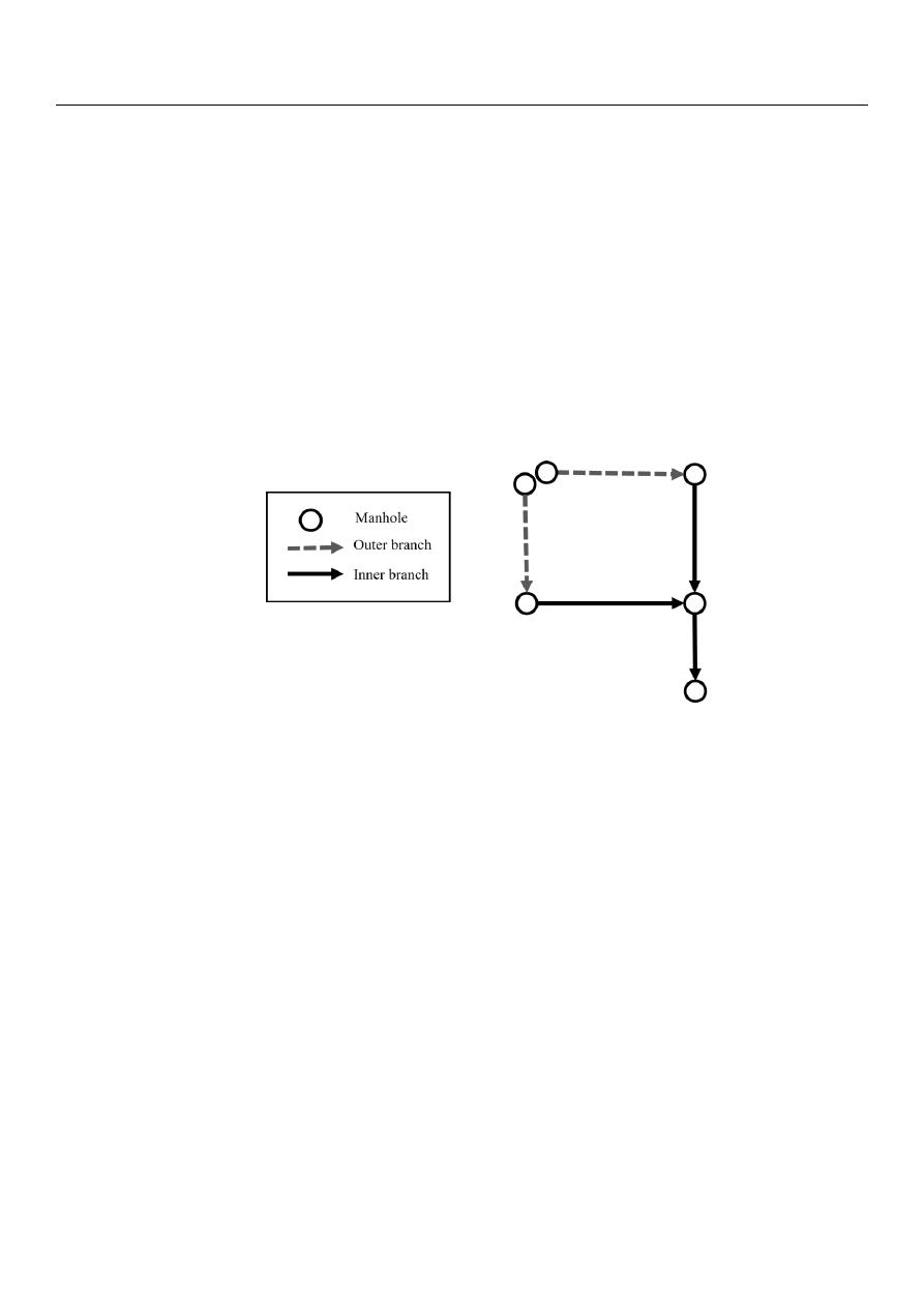
For a layout to be feasible, it cannot allow the recirculation of water through the pipes.
For this reason, a tree-shaped structure is required, that is, a network composed of several
series of pipes with a single discharge. In order to achieve this structure, two types of
pipes are used, outer-branch and inner-branch. An outer-branch pipe is considered to
be the first pipe in a series and receives inflow only from its upstream manhole. On the
contrary, inner-branch pipes are the rest of the pipes in a series. In the model, the pipe type
is represented by the set
T = {
t
1
, t
2
}
, where t
1
represents an outer-branch pipe and a t
2
an
inner-branch pipe. Figure
1
shows a scheme of outer and inner branch pipes.
Water 2021, 13, x FOR PEER REVIEW
3 of 20
2. Background
Since the present work suggests an extension to the methodology proposed by Du-
que et al. [45], the section of background briefly describes what this methodology consists
of.
In the layout selection problem, Duque et al. [45] use MIP to model the drainage sys-
tem as a network design problem that defines the flow direction, flow rate, and connection
type of each pipe that conforms to the sewer network.
The input of the model is an undirected graph composed by a set of nodes ℳ =
{𝑚
1
, … , 𝑚
𝐾
} that represent the manholes of the sewer network, and a set of edges ℰ ⊂
{(𝑚
𝑖
, 𝑚
𝑗
): 𝑚
𝑖
∈ ℳ; 𝑚
𝑗
∈ ℳ; 𝑖 < 𝑗 } that refer to the undirected connection between two
nodes. It is also known the coordinates x, y, and z and the inlet flow from each manhole.
Further, in order to model the directed links between two nodes, that is, pipes with a de-
fined flow direction, a set of arcs is established from the set ℰ. This set is defined as 𝒜
𝐿
=
{(𝑚
𝑖
, 𝑚
𝑗
): (𝑚
𝑖
, 𝑚
𝑗
) ∈ ℰ} ∪ {(𝑚
𝑗
, 𝑚
𝑖
): (𝑚
𝑖
, 𝑚
𝑗
) ∈ ℰ}.
For a layout to be feasible, it cannot allow the recirculation of water through the
pipes. For this reason, a tree-shaped structure is required, that is, a network composed of
several series of pipes with a single discharge. In order to achieve this structure, two types
of pipes are used, outer-branch and inner-branch. An outer-branch pipe is considered to
be the first pipe in a series and receives inflow only from its upstream manhole. On the
contrary, inner-branch pipes are the rest of the pipes in a series. In the model, the pipe
type is represented by the set 𝒯 = {𝑡
1
, 𝑡
2
}, where 𝑡
1
represents an outer-branch pipe and
a 𝑡
2
an inner-branch pipe. Figure 1 shows a scheme of outer and inner branch pipes.
Figure 1. Types of pipes in the sewer network.
The methodology has two decision variables: 𝑥
𝑖𝑗𝑡
, a binary variable that takes the
value of one (1) if the pipe from 𝑚
𝑖
to 𝑚
𝑗
∈ 𝒜
𝐿
, that is of type 𝑡 ∈ 𝒯, is part of the layout
solution; and 𝑞
𝑖𝑗𝑡
, a non-negative real variable that represents the flow rate in the pipe of
type 𝑡 ∈ 𝒯 that goes from 𝑚
𝑖
to 𝑚
𝑗
∈ 𝒜
𝐿
.
Lastly, the decision variables are multiplied by two cost coefficients in the objective
function. These coefficients are 𝑐
𝑖𝑗
, which represents the estimated cost per flow unit that
passes through the pipe from 𝑚
𝑖
to 𝑚
𝑗
; and 𝑎
𝑖𝑗
, which describes the cost associated with
using a pipe with flow direction 𝑚
𝑖
to 𝑚
𝑗
. These costs are estimated by a linear regres-
sion that is updated with the costs obtained in the hydraulic design model. Duque et al.
[45] propose an iterative scheme between the layout selection model and the hydraulic
design model, in which the accuracy of the cost function of the layout selection is im-
proved with each iteration. The disadvantage of this iteration scheme is that it requires
random values of 𝑐
𝑖𝑗
and 𝑎
𝑖𝑗
to start the process, and this affects the convergence of the
algorithm.
The estimated cost of the layout selection model is minimized by Equation (1), which
considers flow rate, flow direction, and pipes required. The weakness of this objective
Figure 1.
Types of pipes in the sewer network.
The methodology has two decision variables: x
ijt
, a binary variable that takes the
value of one (1) if the pipe from m
i
to m
j
∈ A
L
, that is of type t
∈ T
, is part of the layout
solution; and q
ijt
, a non-negative real variable that represents the flow rate in the pipe of
type t
∈ T
that goes from m
i
to m
j
∈ A
L
.
Lastly, the decision variables are multiplied by two cost coefficients in the objective
function. These coefficients are c
ij
, which represents the estimated cost per flow unit that
passes through the pipe from m
i
to m
j
; and a
ij
, which describes the cost associated with
using a pipe with flow direction m
i
to m
j
. These costs are estimated by a linear regression
that is updated with the costs obtained in the hydraulic design model. Duque et al. [
45
]
propose an iterative scheme between the layout selection model and the hydraulic design
model, in which the accuracy of the cost function of the layout selection is improved with
each iteration. The disadvantage of this iteration scheme is that it requires random values
of c
ij
and a
ij
to start the process, and this affects the convergence of the algorithm.
The estimated cost of the layout selection model is minimized by Equation (1), which
considers flow rate, flow direction, and pipes required. The weakness of this objective
function is that it does not include the land topography criterion. This can cause the
selection of layouts that do not match the land slope, especially in non-flat areas.
min
∑
t ∈T
∑
(i,j)∈A
L
c
ij
q
ijt
+
∑
t ∈T
∑
(i,j)∈A
L
a
ij
x
ijt
(1)
According to Haghighi and Bakhshipour [
1
] (p. 790), “in the case of steep basins, based
on engineering judgments it is almost possible to create a cost-effective layout”, this is, for

Water 2021, 13, 2491
4 of 20
sewer networks located in steep topography, an engineer can be guided by the natural land
slope to define a feasible and cost-effective layout. However, the design of the layout is
subjective and depends on the engineer’s experience, especially in flat topography, where
it is not easy to be guided by the natural land slope. Therefore, several layout proposals
are possible, each one of them with its own different cost, some of them being cheaper than
others. In addition, there are many engineering criteria to create the layout, such as: pipes
with higher natural slope, pipes with a greater difference of elevation between manholes,
distance to discharge, number of outer-branch pipes. Therefore, whether steep topography
or not, it is necessary to have a methodology that considers all the components involved in
the layout selection problem.
This research proposes a methodology as an extension of the mathematical optimiza-
tion framework proposed by Duque et al. [
45
], which seeks to solve the layout selection
problem taking into account all the data known in this problem, i.e., land topography,
streets network topology, and inflow to each manhole. This is in order to eliminate the
subjectivity of the layout selection cost function, to obtain a more general methodology
that could be applied to sewer networks with any type of topography, and to decrease
computational effort.
3. Methodology
The present methodology proposes some changes to the objective function of the
layout selection model proposed by Duque et al. [
45
]. First, it is proposed to add a term
to the equation that models the land topography. This term is presented in Equation (2),
where b
ijt
is a coefficient that depends on the land topography in the pipe from m
i
to
m
j
∈ A
L
of type t
∈ T
.
∑
t∈T
∑
(i,j,t)∈A
L
b
ijt
x
ijt
(2)
Another change proposed by the methodology is the way the coefficients c
ij
and
a
ij
are calculated, since Duque et al. [
45
] propose an estimation with linear regression,
but the relation between construction cost and flow rate is not linear. To define the
new values of the coefficients b
ijt
, c
ij
, and a
ij
the methodology proposes two stages: the
selection of an initial layout and an iteration with penalties in excavation. This section
explains those stages.
3.1. Selection of an Initial Layout
To determine the value of the coefficients b
ijt
, c
ij
, and a
ij
an initial hydraulic design
is required, and therefore, an initial layout. Duque et al. [
45
] propose a random initial
layout, but this affects the convergence of the method. Hence, the present methodology
proposes a method to determine an initial layout close to the optimal one based on
engineering criteria.
The method assigns a weight b
ijt
to each pipe, which will be a large value for non-
efficient pipes and, therefore, a small value for the pipes that are desirable on the layout.
Equation (3) defines the objective function of the initial layout, which minimizes the sum
of the weights assigned to the pipes in order to select those with the lowest weight.
min
∑
t∈T
∑
(i,j,t)∈A
L
b
ijt
x
ijt
(3)
Considering that pipes and land slope should be in the same direction in order to
avoid increments in excavation depths, three criteria were proposed to define the value of
the coefficient b
ijt
.
Water 2021, 13, 2491
5 of 20
3.1.1. Criterion 1
This criterion seeks to give priority to the pipes with the same direction of the land
slope by multiplying the slope of the pipe by
−
1. In this way, the pipes that are against
the slope will have a positive b
ijt
and will be discarded from the layout since the objective
function is to be minimized.
Furthermore, this criterion seeks to minimize the number of outer-branch pipes;
therefore, a penalty coefficient µ is assigned to this type of pipe. In order to make the
outer-branch pipes less desirable for the layout selection model, the value of µ should be a
number between 0 and 1 for outer-branch pipes with positive slopes and a value greater
than 1 for outer-branch pipes with negative slopes.
To select the most appropriate value of µ for positive and negative slopes, a sensitivity
analysis was performed. In the analysis, the value of µ for positive slopes ranged between
0.2 and 0.8, while for negative slopes, it ranged between 1.05 and 1.95. Different combina-
tions were tested with these values, and it was concluded that a recommended combination
is 0.65 for positive slopes and 1.65 for negative slopes since designs with the lowest costs
were obtained with these values. However, if another combination of values of µ is chosen
within those tested in the analysis, the change in the cost obtained is approximately 1%. To
resume, the values of µ used are shown in Equation (4).
µ
=
0.65,
s
ijt
1
>
0
1.65,
s
ijt
1
<
0
(4)
where:
s
ijt
1
: is the land slope of the outer-branch pipe from m
i
to m
j
∈ A
L
.
µ
: is the penalty for outer-branch pipes in the selection of the initial layout.
Summarizing, this criterion calculates the coefficient b
ijt
as follows:
b
ijt
2
=
s
ijt
2
∗ (−
1
)
(5)
b
ijt
1
=
s
ijt
1
∗ (−
1
) ∗
µ
(6)
where:
s
ijt
2
: is the land slope of the inner-branch pipe from m
i
to m
j
∈ A
L
.
b
ijt
1
: is the coefficient that depends on the land topography in the outer-branch pipe
from m
i
to m
j
∈ A
L
.
b
ijt
2
: is the coefficient that depends on the land topography in the inner-branch pipe
from m
i
to m
j
∈ A
L
.
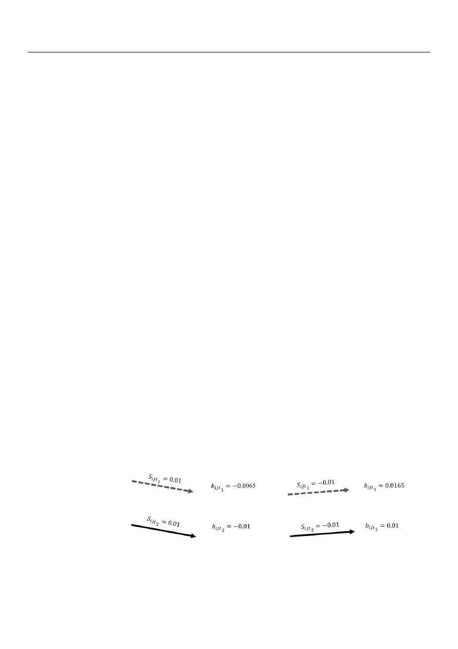
Figure
2
shows an example of how the coefficient b
ijt
is calculated with Criterion 1 in
the two types of pipes with positive and negative slopes. The gray dotted line represents
an outer-branch pipe, where b
ijt
is calculated using Equation (6). On the contrary, the black
continuous line represents an inner-branch pipe, where b
ijt
is calculated using Equation (5).
Water 2021, 13, x FOR PEER REVIEW
6 of 20
Figure 2. Example of the calculation of 𝑏
𝑖𝑗𝑡
with Criterion 1.
3.1.2. Criterion 2
This criterion works the same way as Criterion 1; the slope of each pipe is multiplied
by −1, and the outer-branch pipes are penalized as explained above. However, this crite-
rion also seeks to involve the energy per unit weight or head available to transport the
design flow rate in a pipe and, in this way, prioritize the pipes with greater head or energy
differences. To achieve this, the slope of the pipe is also multiplied by its length, and in
this way, making use of the available head as an input variable. To summarize, with this
criterion, the coefficient 𝑏
𝑖𝑗𝑡
is calculated as follows:
𝑏
𝑖𝑗𝑡
2
= 𝑠
𝑖𝑗𝑡
2
∗ (−1) ∗ 𝐿
𝑖𝑗
(7)
𝑏
𝑖𝑗𝑡
1
= 𝑠
𝑖𝑗𝑡
1
∗ (−1) ∗ 𝐿
𝑖𝑗
∗ 𝜇
(8)
where:
𝐿
𝑖𝑗
: is the length of the pipe from 𝑚
𝑖
to 𝑚
𝑗
∈ ℳ.
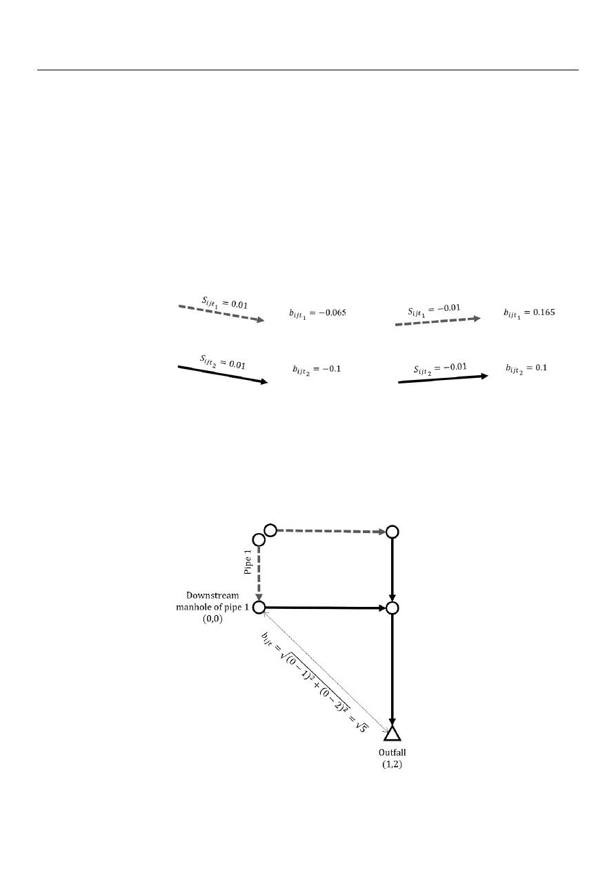
Figure 3 shows an example of how the coefficient 𝑏
𝑖𝑗𝑡
is calculated with Criterion 2
in the two types of pipes with positive and negative slopes, where all pipes are 10 m in
length. In outer-branch pipes the coefficient 𝑏
𝑖𝑗𝑡
is calculated using Equation (8), while in
inner-branch pipes Equation (7) is used.
Figure 3. Example of the calculation of 𝑏
𝑖𝑗𝑡
with Criterion 2.
3.1.3. Criterion 3
With this criterion, the coefficient 𝑏
𝑖𝑗𝑡
is calculated as the Euclidean distance be-
tween the downstream manhole of the pipe, where the weight will be assigned, and the
outfall. This criterion is proposed especially for flat topographies and seeks to minimize
the length of the sewer network main series so that the final excavation depth decreases.
In this criterion, the outer-branch pipes have the same weight as the inner-branch ones.
Figure 4 shows an example of how the coefficient 𝑏
𝑖𝑗𝑡
is calculated with Criterion 3.
Figure 2.
Example of the calculation of b
ijt
with Criterion 1.
3.1.2. Criterion 2
This criterion works the same way as Criterion 1; the slope of each pipe is multiplied
by
−
1, and the outer-branch pipes are penalized as explained above. However, this
criterion also seeks to involve the energy per unit weight or head available to transport the
Water 2021, 13, 2491
6 of 20
design flow rate in a pipe and, in this way, prioritize the pipes with greater head or energy
differences. To achieve this, the slope of the pipe is also multiplied by its length, and in
this way, making use of the available head as an input variable. To summarize, with this
criterion, the coefficient b
ijt
is calculated as follows:
b
ijt
2
=
s
ijt
2
∗ (−
1
) ∗
L
ij
(7)
b
ijt
1
=
s
ijt
1
∗ (−
1
) ∗
L
ij
∗
µ
(8)
where:
L
ij
: is the length of the pipe from m
i
to m
j
∈ M
.
Figure
3
shows an example of how the coefficient b
ijt
is calculated with Criterion 2
in the two types of pipes with positive and negative slopes, where all pipes are 10 m in
length. In outer-branch pipes the coefficient b
ijt
is calculated using Equation (8), while in
inner-branch pipes Equation (7) is used.
Water 2021, 13, x FOR PEER REVIEW
6 of 20
Figure 2. Example of the calculation of 𝑏
𝑖𝑗𝑡
with Criterion 1.
3.1.2. Criterion 2
This criterion works the same way as Criterion 1; the slope of each pipe is multiplied
by −1, and the outer-branch pipes are penalized as explained above. However, this crite-
rion also seeks to involve the energy per unit weight or head available to transport the
design flow rate in a pipe and, in this way, prioritize the pipes with greater head or energy
differences. To achieve this, the slope of the pipe is also multiplied by its length, and in
this way, making use of the available head as an input variable. To summarize, with this
criterion, the coefficient 𝑏
𝑖𝑗𝑡
is calculated as follows:
𝑏
𝑖𝑗𝑡
2
= 𝑠
𝑖𝑗𝑡
2
∗ (−1) ∗ 𝐿
𝑖𝑗
(7)
𝑏
𝑖𝑗𝑡
1
= 𝑠
𝑖𝑗𝑡
1
∗ (−1) ∗ 𝐿
𝑖𝑗
∗ 𝜇
(8)
where:
𝐿
𝑖𝑗
: is the length of the pipe from 𝑚
𝑖
to 𝑚
𝑗
∈ ℳ.
Figure 3 shows an example of how the coefficient 𝑏
𝑖𝑗𝑡
is calculated with Criterion 2
in the two types of pipes with positive and negative slopes, where all pipes are 10 m in
length. In outer-branch pipes the coefficient 𝑏
𝑖𝑗𝑡
is calculated using Equation (8), while in
inner-branch pipes Equation (7) is used.
Figure 3. Example of the calculation of 𝑏
𝑖𝑗𝑡
with Criterion 2.
3.1.3. Criterion 3
With this criterion, the coefficient 𝑏
𝑖𝑗𝑡
is calculated as the Euclidean distance be-
tween the downstream manhole of the pipe, where the weight will be assigned, and the
outfall. This criterion is proposed especially for flat topographies and seeks to minimize
the length of the sewer network main series so that the final excavation depth decreases.
In this criterion, the outer-branch pipes have the same weight as the inner-branch ones.
Figure 4 shows an example of how the coefficient 𝑏
𝑖𝑗𝑡
is calculated with Criterion 3.
Figure 3.
Example of the calculation of b
ijt
with Criterion 2.
3.1.3. Criterion 3
With this criterion, the coefficient b
ijt
is calculated as the Euclidean distance between
the downstream manhole of the pipe, where the weight will be assigned, and the outfall.
This criterion is proposed especially for flat topographies and seeks to minimize the length
of the sewer network main series so that the final excavation depth decreases. In this
criterion, the outer-branch pipes have the same weight as the inner-branch ones.
Figure
4
shows an example of how the coefficient b
ijt
is calculated with Criterion 3.
Water 2021, 13, x FOR PEER REVIEW
7 of 20
Figure 4. Example of the calculation of 𝑏
𝑖𝑗𝑡
with Criterion 3.
With the criteria explained above, three different layouts are obtained, one with each
criterion. The one with the lowest cost is chosen as the initial layout. Then, the coefficients
𝑐
𝑖𝑗
and 𝑎
𝑖𝑗
are calculated to run the iteration with penalties in excavation. This process
will be explained in the next section.
3.2. Iteration with Penalties in Excavation
Duque et al. [45] proposed to determine the value of 𝑐
𝑖𝑗
and 𝑎
𝑖𝑗
through a linear
regression between the total cost of a pipe and its design flow rate. However, this meth-
odology has two problems. First, the outer-branch pipes are included in the linear regres-
sion. This means that a big part of the data is concentrated in the intercept, where costs
and design flow rates are low. Second, the length of the pipes is not considered in the
linear regression because it relates the flow rate of a pipe to its total cost, not the cost per
unit length. This means that costs with different magnitudes are related to the same flow
rate in the regression.
For the first problem, this paper proposes not to include the outer-branch pipes in
the linear regression since most of the time, this type of pipe uses the minimum diameter
and excavation depth. This means that, generally, the cost per unit length is the same for
every outer-branch pipe. For this reason, the cost of these pipes can be determined only
by the coefficient 𝑏
𝑖𝑗𝑡
, which means that coefficients 𝑐
𝑖𝑗
and 𝑎
𝑖𝑗
are zero for these pipes.
With the initial layout, an initial hydraulic design is obtained, and in this way, it is
possible to determine the average cost per unit length of the outer-branch pipes and the
cost that will be assigned to the arcs of the layout selection model in the next iteration.
The above applies when the land slope is greater than or equal to the average instal-
lation slope of the outer-branch pipes in the previous iteration. If this is not the case, the
excavation depth of the downstream manhole may become greater, which causes an in-
crease in the construction cost. This increment in cost is considered by a penalty in the
coefficient 𝑏
𝑖𝑗𝑡
and is calculated as the cost of the extra excavated volume based on the
diameter and slope of the pipes from the initial layout, the natural land slope, and the cost
function from the hydraulic design model. Equation (9) defines the value of 𝑏
𝑖𝑗𝑡
for outer-
branch pipes in the iteration with penalties in excavation.
Figure 4.
Example of the calculation of b
ijt
with Criterion 3.

Water 2021, 13, 2491
7 of 20
With the criteria explained above, three different layouts are obtained, one with each
criterion. The one with the lowest cost is chosen as the initial layout. Then, the coefficients
c
ij
and a
ij
are calculated to run the iteration with penalties in excavation. This process will
be explained in the next section.
3.2. Iteration with Penalties in Excavation
Duque et al. [
45
] proposed to determine the value of c
ij
and a
ij
through a linear regres-
sion between the total cost of a pipe and its design flow rate. However, this methodology
has two problems. First, the outer-branch pipes are included in the linear regression.
This means that a big part of the data is concentrated in the intercept, where costs and
design flow rates are low. Second, the length of the pipes is not considered in the linear
regression because it relates the flow rate of a pipe to its total cost, not the cost per unit
length. This means that costs with different magnitudes are related to the same flow rate in
the regression.
For the first problem, this paper proposes not to include the outer-branch pipes in the
linear regression since most of the time, this type of pipe uses the minimum diameter and
excavation depth. This means that, generally, the cost per unit length is the same for every
outer-branch pipe. For this reason, the cost of these pipes can be determined only by the
coefficient b
ijt
, which means that coefficients c
ij
and a
ij
are zero for these pipes.
With the initial layout, an initial hydraulic design is obtained, and in this way, it is
possible to determine the average cost per unit length of the outer-branch pipes and the
cost that will be assigned to the arcs of the layout selection model in the next iteration.
The above applies when the land slope is greater than or equal to the average in-
stallation slope of the outer-branch pipes in the previous iteration. If this is not the case,
the excavation depth of the downstream manhole may become greater, which causes an
increase in the construction cost. This increment in cost is considered by a penalty in the
coefficient b
ijt
and is calculated as the cost of the extra excavated volume based on the
diameter and slope of the pipes from the initial layout, the natural land slope, and the
cost function from the hydraulic design model. Equation (9) defines the value of b
ijt
for
outer-branch pipes in the iteration with penalties in excavation.
b
ijt
1
=
C
t
1
∗
L
ij
, s
ijt
1
≥
S
t
1
C
t
1
∗
L
ij
+
γ
ij
, s
ijt
1
<
S
t
1
(9)
where:
C
t
1
: is the average cost per unit length of outer-branch pipes.
S
t
1
: is the average installation slope of outer-branch pipes.
γ
ij
: is the penalty for increments in excavation cost in pipe from m
i
to m
j
∈ A
L
.
For the second problem of the methodology proposed by Duque et al. [
45
], that
is, not considering the effect of the pipes’ length in the linear regression, this article
proposes to perform the regression between the costs per unit length and the flow rate
of each inner-branch pipe, where c
ij
is equivalent to the slope of the linear equation and
a
ij
to the intercept.
Similar to outer-branch pipes, when the sewer network is located on steep terrain,
there is a possibility that the methodology selects inner-branch pipes that are against the
natural land slope to try to minimize the cost per flow unit. In this case, there is the problem
again of obtaining pipes with greater excavation depths. This should be considered in
the model the same way that with outer-branch pipes, this is, with the penalty for the
increments in excavation costs.
Unlike outer-branch pipes, when the land slope is greater than the average installation
slope, the depth of the upstream manhole may decrease. This implies a cost reduction
associated with less excavation depth required, and it also should be considered in the
coefficient b
ijt
through a bonus that is calculated as the cost of the excavation depth
multiplied by
−
1.

Water 2021, 13, 2491
8 of 20
In other words, for inner-branch pipes, the coefficient b
ijt
must include a bonus or
penalty depending on the land slope and the average installation slope of these pipes.
Equations (10) and (11) define the value of b
ijt
for this type of pipe as explained above.
b
ijt
2
=
ω
ij
, s
ijt
2
≥
S
t
2
γ
ij
, d.l.c.
(10)
ω
ij
= −
γ
ij
(11)
where:
S
t
2
: is the average installation slope of inner-branch pipes.
ω
ij
: is the bonus for reduction in excavation cost in pipe from m
i
to m
j
∈ A
L
.
Unlike the methodology proposed by Duque et al. [
45
], the current methodology does
not require several iterations because if the procedure performed in the iteration with
penalties in excavation is repeated, similar coefficients b
ijt
will be obtained. Therefore,
computational time will be greater and similar designs will be obtained and not necessarily
with lower costs. On the other hand, the iteration with penalties in excavation does not
always manage to reduce the costs of the sewer network design; sometimes the use of
Criteria 1, 2 and 3 is sufficient to obtain the design with the lowest cost.
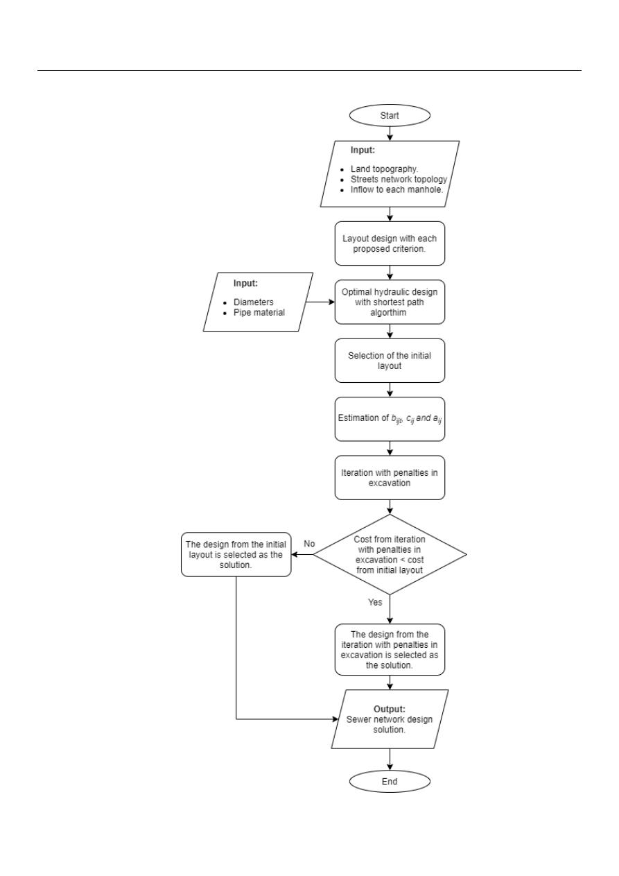
To resume, in the iteration scheme proposed in the present work, first, a sewer network
design is obtained with each criterion; then, the initial layout is selected, which is the one
with the lowest cost. Next, with the selected initial layout, the coefficients b
ijt
, c
ij
, and
a
ij
are estimated and the iteration with penalties in excavation is performed. Finally, the
design obtained with the initial layout and the one obtained with the penalties in the
excavation are compared to select the design with the lowest cost as the solution. The
above is summarized in Figure
5
.
3.3. Case Studies
To compare the proposed approach with others found in the literature, the method-
ology was tested in three sewer networks. Each of them is composed of a number of
manholes and pipes that are established by the street topology. Additionally, in each man-
hole, there is an inlet flow and the sum of these forms the total flow rate. This information
is part of the input data of the model and is described below for each case study.
The first network was proposed by Li and Matthew [
34
]; it is composed of 57 manholes
and 79 pipes, has a flat topography, and a total flow rate of 0.338 m
3
/s. The second sewer
network was proposed by Moeini and Afshar [
46
]; it has 81 manholes, 144 pipes, a total
flow rate of 0.593 m
3
/s, and its topography is completely flat since each manhole has the
same elevation. The third sewer network is called Chicó and was proposed by Duque
et al. [
45
]; it is part of a real sewer network located in Bogotá, Colombia. It has 109 manholes,
160 pipes, it is located in wavy topography terrain, and the total flow rate is 1.526 m
3
/s.
Table
1
presents the hydraulic constrains used in the three designs. For the velocity
calculation, Manning’s equation was used with a coefficient n
=
0.014 (concrete). The set
diameters, in meters, used are D
=
{
0.2, 0.25, 0.3, 0.35, 0.38, 0.4, 0.45, 0.5, 0.53, 0.6, 0.7,
0.8, 0.9, 1.0, 1.05, 1.20, 1.35, 1.4, 1.5, 1.6, 1.8, 2, 2.2, 2.4
}
. The elevation change utilized was
∆Z
=
0.1 m, because in a 100-m-long pipe, this is the elevation that allows a 0.001 slope,
which is the minimum buildable slope.
Water 2021, 13, 2491
9 of 20
Water 2021, 13, x FOR PEER REVIEW
9 of 20
Figure 5. Methodology flow chart.
Figure 5.
Methodology flow chart.

Water 2021, 13, 2491
10 of 20
Table 1.
Hydraulic constraints.
Constraint
Value
Condition
Minimum diameter
0.2 m
Always
Maximum filling ratio
0.6
d
≤
0.3 m
0.7
0.35 m
≤
d
≤
0.45 m
0.75
0.5 m
≤
d
≤
0.9 m
0.8
d
≥
1 m
Minimum velocity
0.7 m/s
d
≤
0.5 m and Flow rate
>
0.015 m
3
/s
0.8 m/s
d
>
0.5 m and Flow rate
>
0.015 m
3
/s
Maximum velocity
5 m/s
Always
Minimum gradient
0.003
Flow rate
<
0.015 m
3
/s
Minimum depth
1 m
Always
To compare the designs with previous designs, two cost functions were used.
The first cost function was proposed by Li and Matthew [
34
], and it is presented in
Equations (12) and (13), where f
p
and f
m
are the construction cost in yuan for a pipe
and a manhole, respectively.
f
p
=
4.27
+
93.59d
2
+
2.86dh
+
2.39h
2
L
i f d
≤
1 m and h
≤
3 m
36.47
+
88.96d
2
+
8.70dh
+
1.78h
2
L
i f d
≤
1 m and h
>
3 m
20.50
+
149.27d
2
−
58.96dh
+
17.75h
2
L
i f d
>
1 m and h
≤
4 m
78.44
+
29.25d
2
+
31.80dh
−
2.32h
2
L
i f d
>
1 m and h
>
4 m
(12)
f
m
=
136.67
+
166.19d
2
+
3.50dh
+
16.22h
2
i f d
≤
1 m and h
≤
3 m
132.91
+
790.94d
2
−
280.23dh
+
34.97h
2
i f d
≤
1 m and h
>
3 m
209.74
+
57.53d
2
+
10.93dh
+
19.88h
2
i f d
>
1 m and h
≤
4 m
210.66
−
113.04d
2
+
126.43dh
−
0.60h
2
i f d
>
1 m and h
>
4 m
(13)
In Equations (12) and (13), d is the pipe diameter (m), h is the pipe average buried
depth (m), and L is the pipe length (m).
The second cost function used was proposed by Maurer, Wolfram, and Anja [
47
]. This
is presented in Equations (14)–(16).
C
= (
αh
+
β
) ∗
L
(14)
α
=
m
α
d
+
n
α
(15)
β
=
m
β
d
+
n
β
(16)
where C is the pipe construction cost in USD, L is the pipe length (m), α is a coefficient
related to the excavation depth cost (USD*m
−2
), h is the buried depth (m), β is the pipe cost
per unit length (USD*m
−1
), m
α
, m
β
, n
α
, and n
β
are constants and their values are presented
in Table
2
.
Table 2.
Constants of the cost function proposed by Maurer et al. [
47
].
Constant
Value
Units
m
α
110
USD
∗
m
−3
m
β
1200
USD
∗
m
−2
n
α
127
USD
∗
m
−2
n
β
−
35
USD
∗
m
−1

Water 2021, 13, 2491
11 of 20
4. Results
For each sewer network, Criteria 1, 2, and 3 were applied to obtain three different
layouts. Then, for each network, the layout with the lowest cost was selected to
estimate the value of coefficient b
ijt
, the penalties, and bonuses. Lastly, the iteration
with penalties in the excavation was run to try to obtain a lower cost than the cost
obtained with the initial layout.
4.1. Benchmark Network Proposed by Li and Matthew
Table
3
presents the construction cost obtained with the cost function of Li and
Matthew [
34
] and Maurer et al. [
47
].
Table 3.
Construction cost for each criterion in the benchmark proposed by Li and Matthew [
34
].
Scenario
Construction Cost
×
10
6
(CNY)
Function of Li and Matthew [
34
]
Construction Cost
×
10
6
(USD)
Function of Maurer et al. [
47
]
Criterion 1
1.36
20.06
Criterion 2
1.33
19.91
Criterion 3
1.42
19.58
For the cost function of Li and Matthew, the design obtained with Criterion 2 has the
lowest cost. On the other hand, for the cost function of Maurer et al., the design with the
lowest cost is the one obtained with Criterion 3. The layouts of these designs are selected
as the initial layouts, and with these layouts, the iteration with penalties in the excavation
was calculated. The construction cost obtained in the iteration with penalties in excavation
with the cost function of Li and Matthew was CNY 1.12
×
10
6
and with the cost function of
Maurer et al. was USD 17.01
×
10
6
. In both cases, the cost was reduced with the iteration
with penalties in excavation.
Table
4
presents the construction cost achieved with the function of Li and Matthew
with different methodologies proposed in the literature.
Table 4.
Construction cost with different methods for the benchmark proposed by Li and Matthew [
34
].
Method
Researchers
Construction Cost
×
10
6
(CNY)
Function of Li and Matthew [
34
]
MGA
Pan and Kao [
32
]
1.91
Adaptative GA
Haghighi and Bakhshipour [
20
]
1.84
Loop-by-loop cutting algorithm and GA-DDDP
Haghighi and Bakhshipour [
35
]
1.59
SDE-GOBL
Liu, Han, Wang, and Qiao [
48
]
1.53
Loop-by-loop cutting algorithm and TS
Haghighi and Bakhshipour [
28
]
1.43
Reliability-DDDP
Haghighi and Bakhshipour [
1
]
2.41
MILP
Safavi and Geranmehr [
7
]
1.57
ACOA-TGA-NLP
Moeini and Afshar [
46
]
1.39
MIP and DP
Duque et al. [
45
]
1.29
MIP and DP Extension
Present work
1.12
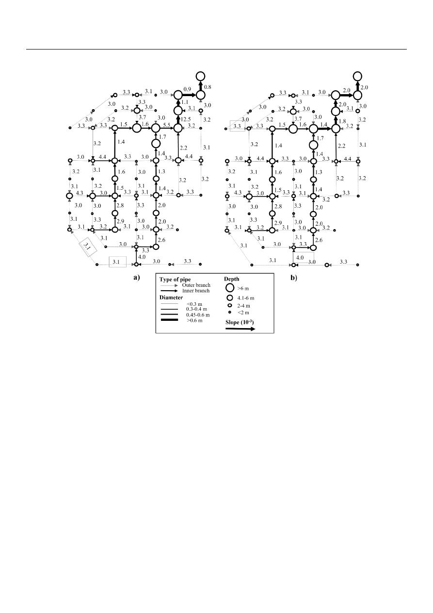
Figure
6
shows the designs for the lowest costs obtained with the cost function of Li
and Matthew and with the cost function of Maurer et al. in the benchmark network pro-
posed by Li and Matthew. The depth shown corresponds to the invert depth of manholes.
This depth is with respect to the ground level on the manhole location. This notation does
not mean that a pipe can go from a deeper to a shallower manhole because it is not taking
into account the ground levels. This also applies to Figures
7
and
8
.
Water 2021, 13, 2491
12 of 20
Water 2021, 13, x FOR PEER REVIEW
12 of 20
Table 4. Construction cost with different methods for the benchmark proposed by Li and Matthew [34].
Method
Researchers
Construction Cost × 10
6
(CNY)
Function of Li and Matthew [34]
MGA
Pan and Kao [32]
1.91
Adaptative GA
Haghighi and Bakhshipour [20]
1.84
Loop-by-loop cutting algorithm and GA-
DDDP
Haghighi and Bakhshipour [35]
1.59
SDE-GOBL
Liu, Han, Wang, and Qiao [48]
1.53
Loop-by-loop cutting algorithm and TS
Haghighi and Bakhshipour [28]
1.43
Reliability-DDDP
Haghighi and Bakhshipour [1]
2.41
MILP
Safavi and Geranmehr [7]
1.57
ACOA-TGA-NLP
Moeini and Afshar [46]
1.39
MIP and DP
Duque et al. [45]
1.29
MIP and DP Extension
Present work
1.12
Figure 6 shows the designs for the lowest costs obtained with the cost function of Li
and Matthew and with the cost function of Maurer et al. in the benchmark network pro-
posed by Li and Matthew. The depth shown corresponds to the invert depth of manholes.
This depth is with respect to the ground level on the manhole location. This notation does
not mean that a pipe can go from a deeper to a shallower manhole because it is not taking
into account the ground levels. This also applies to Figures 7 and 8.
Figure 6. Scheme (not to scale) of the best design of the benchmark network proposed by Li and Matthew [34] with (a)
their cost function and (b) the cost function of Maurer et al. [47].
Figure 6.
Scheme (not to scale) of the best design of the benchmark network proposed by Li and Matthew [
34
] with (a) their
cost function and (b) the cost function of Maurer et al. [
47
].
4.2. Benchmark Network Proposed by Moeini and Afshar
To apply Criteria 1 and 2, it is necessary to have a pipe slope different from zero,
which does not happen in the Moeini and Afshar network because originally, it was totally
flat. For this reason, to apply Criteria 1 and 2, the manhole elevations were modified so that
instead of a flat terrain, a small slope (0.001) was used for the layout selection. This was
done only to obtain the layout, and then, in the hydraulic design, the original elevations
were used, i.e., 1000 m for each manhole.
Table
5
presents the costs obtained with the different criteria and cost functions.
In this sewer network, designs with lower costs were obtained with Criterion 2 for
both cost functions, and in the iteration with penalties in excavation, the cost achieved was
CNY 38.45
×
10
4
with the cost function of Li and Matthew, and USD 845.08
×
10
4
with the
cost function of Maurer et al. The iteration with penalties in excavation did not reduce
the cost of the designs; therefore, the best designs are those obtained with Criterion 2.
Table
6
presents the comparison of construction cost between different methods for this
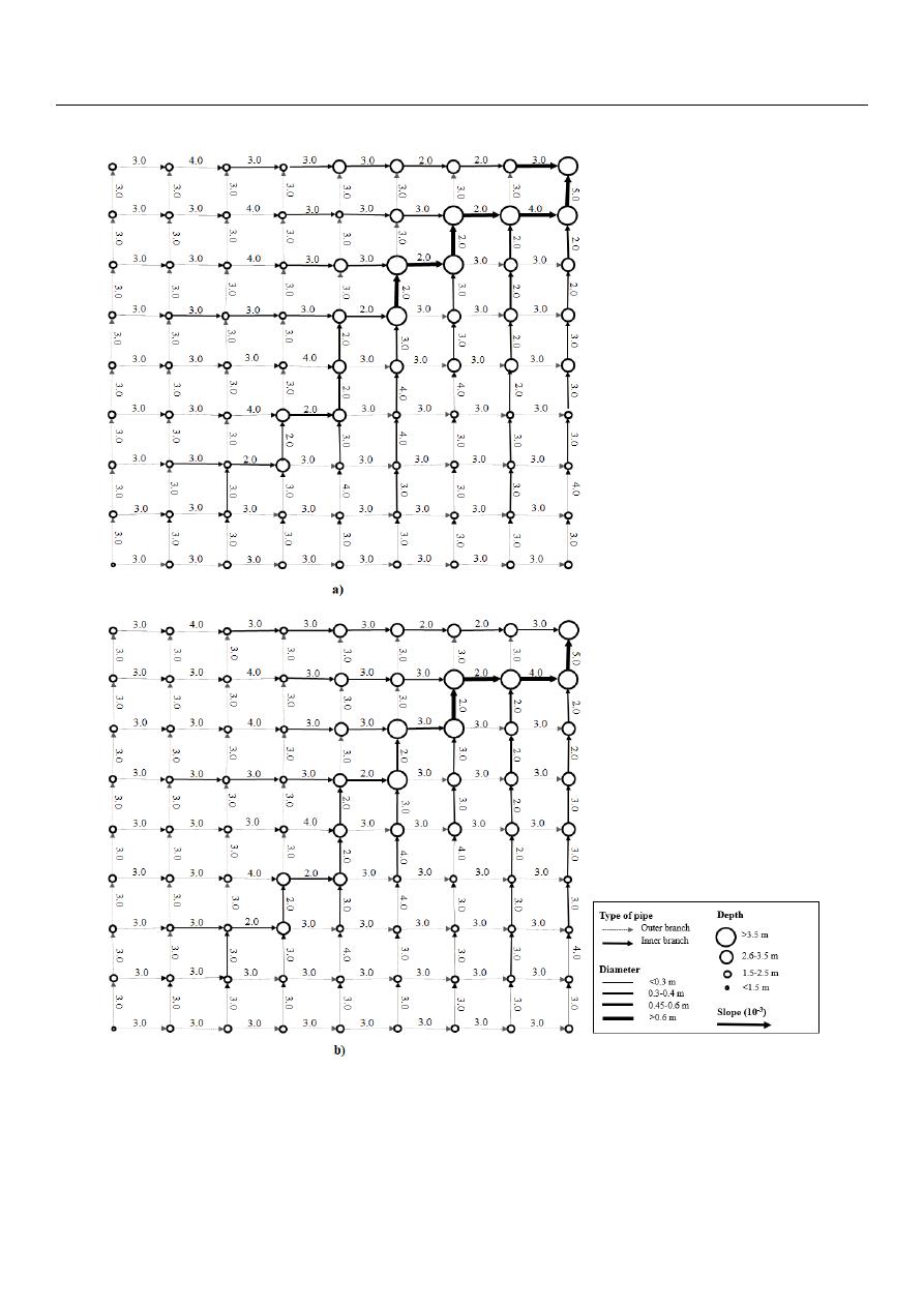
sewer network, and Figure
7
shows the designs with the lowest cost obtained with the cost
function of Li and Matthew and with the cost function of Maurer et al.
Water 2021, 13, 2491
13 of 20
Water 2021, 13, x FOR PEER REVIEW
13 of 20
Figure 7. Scheme (not to scale) of the best design of the benchmark network proposed by Moeini and Afshar [46] with (a)
the cost function of Li and Matthew [34] and (b) the cost function of Maurer et al. [47].
Figure 7.
Scheme (not to scale) of the best design of the benchmark network proposed by Moeini and Afshar [
46
] with
(a) the cost function of Li and Matthew [
34
] and (b) the cost function of Maurer et al. [
47
].
Water 2021, 13, 2491
14 of 20
Water 2021, 13, x FOR PEER REVIEW
14 of 20
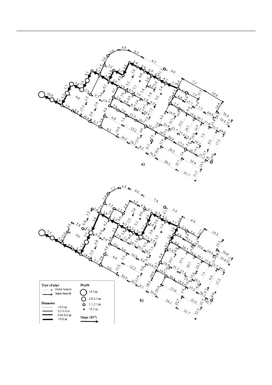
Figure 8. Scheme (not to scale) of the best design of the benchmark network proposed by Duque et al. [45] with (a) the cost
function of Li and Matthew [34] and (b) the cost function of Maurer et al. [47].
Figure 8.
Scheme (not to scale) of the best design of the benchmark network proposed by Duque et al. [
45
] with (a) the cost
function of Li and Matthew [
34
] and (b) the cost function of Maurer et al. [
47
].

Water 2021, 13, 2491
15 of 20
Table 5.
Construction cost for each criterion in the benchmark proposed by Moeini and Afshar [
46
].
Scenario
Construction Cost
×
10
4
(CNY)
Function of Li and Matthew [
34
]
Construction Cost
×
10
4
(USD)
Function of Maurer et al. [
47
]
Criterion 1
36.86
817.83
Criterion 2
35.99
813.46
Criterion 3
45.55
862.07
Table 6.
Construction cost with different methods for the benchmark proposed by Moeini and Afshar [
46
].
Method
Researchers
Construction Cost
×
10
4
(CNY)
Function of Li and Matthew [
34
]
ACOA-TGA-NLP
Moeini and Afshar [
46
]
64.08
MIP and DP
Duque et al. [
45
]
36.95
MIP and DP Extension
Present work
35.99
4.3. Benchmark Network Proposed by Duque et al.: Chicó
In the sewer network Chicó, the lowest cost was achieved with Criterion 2 using the
Li and Matthew function and with Criterion 1 using the Maurer et al. function. Table
7
presents the cost obtained with each criterion.
Table 7.
Construction cost for each criterion in the benchmark proposed by Duque et al. [
45
].
Scenario
Construction Cost
×
10
4
(CNY)
Function of Li and Matthew [
34
]
Construction Cost
×
10
4
(USD)
Function of Maurer et al. [
47
]
Criterion 1
38.22
843.38
Criterion 2
38.12
856.89
Criterion 3
60.01
1093.93
After running the iteration with penalties in excavation, the cost obtained was
CNY 39.04
×
10
4
with the cost function of Li and Matthew and USD 886.87
×
10
4
with
the cost function of Maurer et al.; this means the iteration with penalties in excavation
did not achieve a lower cost. Consequently, the best designs are the ones found in
the initial layout stage. Table
8
compares this cost with the cost achieved by Duque
et al. [
1
].
Table 8.
Construction cost with different methods for the benchmark proposed by Duque et al. [
45
].
Method
Researchers
Construction Cost
×
10
4
(CNY)
Function of Li and Matthew [
34
]
Maximum Excavation
Depth (m)
Outfall Diameter (m)
MIP and DP
Duque et al. [
45
]
69.91
15.9
1.05
MIP and DP
Extension
Present work
38.12
4.5
0.9
Figure
8
shows the designs with the lowest cost obtained with the cost function of Li
and Matthew and with the cost function of Maurer et al.
The input data and the detailed hydraulic design of each sewer network tested can be
found in the Supplementary Material.
4.4. Computational Effort
In order to compare the computational effort in the methodology proposed by Duque
et al. [
45
] and the current methodology, Table
9
shows the iterations and computational time
used with each approach in each case study with the cost function of Li and Matthew and

Water 2021, 13, 2491
16 of 20
an elevation change of
∆Z
=
0.1 m. In MIP and DP Extension, three of the four iterations
correspond to the three different designs obtained with each criterion describing land
topography, and the other iteration corresponds to the one with penalties in excavation.
Table 9.
Computational effort in MIP and DP, and MIP and DP Extension.
MIP and DP
(Duque et al. [
1
])
MIP and DP Extension
(Present work)
Benchmark Network
Iterations (-)
Time (min)
Iterations (-)
Time (min)
Li and Matthew [
34
]
10
45
4
5
Moeini and Afshar [
46
]
30
115
4
12
Duque et al. [
45
]: Chicó
25
113
4
7
5. Discussion
In all three case studies, the proposed methodology achieved designs with lower
costs than previously reported in the literature. This demonstrates the importance of
incorporating the land topography criterion into the layout selection model, especially in
very-flat or non-uniform terrain, where it is difficult for an engineer to select the optimal
layout or one close to it.
The most significant cost reduction was obtained in the sewer network Chicó.
This is mainly due to the decrease in the maximum excavation depth. This shows that
considering the land topography achieves very satisfactory results in sewer networks
located on wavy or non-flat topography. On the other hand, in the sewer network of
Moeini and Afshar, it was more difficult to apply the methodology due to the change in
elevations that had to be made since it is a hypothetical sewer network without slope.
Although this network also managed to improve the costs reported in the literature, the
cost reduction was not as significant.
Comparing the methodology proposed by Duque et al. [
45
] with the proposal in
this paper, it can be seen that the construction cost of the sewer networks tested was
reduced. In addition, this was achieved with a much shorter computational effort, since
the methodology of Duque et al. [
45
] used between 10 and 30 iterations per network, while
in this methodology, only four iterations per network are necessary, three for the selection
of the initial layout and another one for the iteration with penalties in excavation. As for
computational time, this was reduced by approximately 88% in the Li and Matthew, and
Moeini and Afshar benchmark networks, and by about 94% in the Chicó network.
Achieving the design of a sewer network that complies with hydraulic restrictions
and has a lower construction cost is important, especially for populations that have a
limited budget and that often opt for cheaper alternatives that do not meet all the necessary
restrictions for proper hydraulic operation. In addition, having cheaper sewer networks
designs favors achieving equitable and adequate access to sanitation services, which is one
of the targets related to Sustainable Development Goal 6 (Clean Water and Sanitation) [
49
].
6. Conclusions
This article proposes an objective function for the layout selection problem of a sewer
network system that considers all the variables known in this problem, such as: land
topography, streets network topology, and inflows to each manhole.
To apply the proposed function, two stages are needed. The first one consists of the
selection of an initial layout and its hydraulic design. This initial layout is determined
through criteria that seek to follow the topography of the area. The hydraulic design of the
initial layout is carried out according to the methodology proposed by Duque et al. [
45
],
which guarantees global optimality.
The second stage consists of penalizing the excavation of the pipes and determining
the coefficients of the proposed objective function so that an accurate approximation of the

Water 2021, 13, 2491
17 of 20
construction cost of each arc of the layout selection problem can be made. This is in order
to try to achieve lower costs than in the first stage.
The methodology was tested in three benchmarks using two cost functions pro-
posed by Li and Matthew [
34
] and Maurer et al. [
47
]. The cost obtained with the function
of Li and Matthew was used to compare the designs obtained with the designs of other
methodologies of the literature. With the results obtained, the following conclusions
were made:
•
In the three case studies tested, the present methodology achieved the lowest con-
struction cost reported in the literature. The cost reduction was more significant in the
network with wavy topography, i.e., Chicó. While in the other networks, which are
flat, the cost reduction was not so big, especially in the Moini and Afshar network,
which is completely flat.
•
The cost reduction was achieved in fewer iterations and in significantly less computa-
tional time when compared to the methodology of Duque et al. [
1
]. This shows that
when selecting an optimal layout or one close to it, it is only required to perform the
shortest path algorithm once to obtain a cost-effective sewer network design.
•
Land topography turned out to be an important input in the layout selection model
since whether the land topography is flat or not, a layout that follows the land slope
and maximizes the number of inner-branch pipes allows a cost-effective layout to be
obtained.
In future research, the current methodology could be easily extended to include drop
manholes in hilly terrains and pumping stations in very flat terrains. Moreover, other cost
functions could be used in the layout selection problem, such as nonlinear equations, to
represent more accurately the construction costs of each arc. Further, in the future, the
resilience of the sewer network should be considered in a multi-objective optimization
scheme, as well as consider the possibility of dividing the layout to increase the resilience
of the system.
Supplementary Materials:
The following are available online at
https://www.mdpi.com/article/10
.3390/w13182491/s1
, Table S1: Input data of the benchmark proposed by Li and Matthew [
34
], Table
S2: Hydraulic design for the benchmark proposed by Li and Matthew [
34
] with cost function of Li
and Matthew [
34
], Table S3: Hydraulic design for the benchmark proposed by Li and Matthew [
34
]
with cost function of Maurer et al. [
47
], Table S4: Input data benchmark proposed by Moeini and
Afshar [
46
], Table S5: Hydraulic design for the benchmark proposed by Moeini and Afshar [
46
] with
cost function of Li and Matthew [
34
], Table S6: Hydraulic design for the benchmark proposed by
Moeini and Afshar [
46
] with cost function of Maurer et al. [
47
], Table S7: Input data benchmark
proposed by Duque et al.: Chicó [
45
], Table S8: Hydraulic design for the benchmark proposed by
Duque et al.: Chicó [
45
] with cost function of Li and Matthew [
34
], Table S9: Hydraulic design for the
benchmark proposed by Duque et al.: Chicó [
45
] with cost function of Maurer et al. [
47
].
Author Contributions:
Conceptualization, J.S. and J.Z.; methodology, J.S. and J.H.; software, J.Z.;
validation, J.S., J.H. and P.L.I.-R.; formal analysis, J.S. and J.H; investigation, J.S., J.Z, J.H. and P.L.I.-R.;
writing—original draft preparation, J.Z. and J.H.; writing—review and editing, J.S., J.H. and P.L.I.-R.
All authors have read and agreed to the published version of the manuscript.
Funding:
This research received no external funding.
Conflicts of Interest:
The authors declare no conflict of interest.

Water 2021, 13, 2491
18 of 20
Nomenclature
From methodology proposed by Duque et al. [
45
]:
M
set of nodes representing manholes.
E
set of undirected edges representing links between two nodes m
i
∈ M
; m
j
∈ M
.
A
L
set of directed links between two manholes, m
i
and m
j
, so that (m
i
, m
j
) ∈ E
.
T
set of possible types of pipes, containing outer-branch pipes (t
1
) and inner-branch
pipes (t
2
).
x
ijt
binary decision variable that represents the flow direction and connection type in
the network layout, for all (m
i
, m
j
) ∈ A
L
and t
∈
T.
q
ijt
continuous decision variable that represents the flow through arc m
i
, m
j
)
of type t,
for all for all (m
i
, m
j
) ∈ A
L
and t
∈
T.
a
ij
fixed cost estimate for selecting the flow direction m
i
to m
j
.
c
ij
estimation of cost per flow unit that traverses from m
i
to m
j
.
From present methodology:
b
ijt
coefficient that depends on the land topography in the pipe from m
i
to m
j
∈ A
L
of
type t
∈ T
.
s
ijt
land slope in the pipe from m
i
to m
j
∈ A
L
of type t
∈ T
.
S
t
1
average installation slope of outer-branch pipes.
S
t
2
average installation slope of inner-branch pipes.
L
ij
length of the pipe from m
i
to m
j
∈ M
.
C
t
1
average cost per unit length of outer-branch pipes.
µ
penalty for outer-branch pipes in the selection of the initial layout.
γ
ij
penalty for increments in excavation cost in pipe from m
i
to m
j
∈ A
L
.
ω
ij
bonus for reduction in excavation cost in pipe from m
i
to m
j
∈ A
L
.
References
1.
Haghighi, A.; Bakhshipour, A. Reliability-based layout design of sewage collection systems in flat areas. Urban Water J. 2015, 13,
790–802. [
CrossRef
]
2.
Holland, M.E. Computer Models of Waste-Water Collection Systems. Ph.D. Thesis, Harvard University, Cambridge, MA, USA,
May 1966.
3.
Dajani, J.S.; Hasit, Y. Capital cost minimization of drainage networks. J. Environ. Eng. Div. 1974, 100, 325–337. [
CrossRef
]
4.
Deininger, R.A. Computer aided design of waste collection and treatment systems. In Proceedings of the 2nd Annual Conference
of American Water Resources, Chicago, IL, USA, 18 May 1966; pp. 247–258.
5.
Elimam, A.A.; Charalambous, C.; Ghobrial, F.H. Optimum design of large sewer networks. J. Environ. Eng. 1989, 115, 1171–1190.
[
CrossRef
]
6.
Gupta, M.; Rao, P.; Jayakumar, K. Optimization of integrated sewerage system by using simplex method. VFSTR J. Stem. 2017, 3,
2455–2062.
7.
Safavi, H.; Geranmehr, M.A. Optimization of sewer networks using the mixed-integer linear programming. Urban Water J. 2016,
14, 452–459. [
CrossRef
]
8.
Swamee, P.K.; Sharma, A.K. Optimal design of a sewer line using linear programming. Appl. Math. Model. 2013, 37, 4430–4439.
[
CrossRef
]
9.
Mansouri, M.; Khanjani, M. Optimization of sewer networks using nonlinear programming. J. Water Wastewater 1999, 10, 20–30.
10.
Price, R.K. Design of storm water sewers for minimum construction cost. In Proceedings of the 1st International Conference on
Urban Storm Drainage, Southampton, UK, 1 January 1978; pp. 636–647.
11.
Swamee, P.K. Design of Sewer Line. J. Environ. Eng. 2001, 127, 776–781. [
CrossRef
]
12.
Gupta, A.; Mehndiratta, S.L.; Khanna, P. Gravity Wastewater Collection Systems Optimization. J. Environ. Eng. 1983, 109,
1195–1209. [
CrossRef
]
13.
Kulkarni, V.S.; Khanna, P. Pumped Wastewater Collection Systems Optimization. J. Environ. Eng. 1985, 111, 589–601. [
CrossRef
]
14.
Mays, L.W.; Yen, B.C. Optimal cost design of branched sewer systems. Water Resour. Res. 1975, 11, 37–47. [
CrossRef
]
15.
Walters, G.A. The design of the optimal layout for a sewer network. Eng. Optim. 1985, 9, 37–50. [
CrossRef
]
16.
Walters, G.A.; Templeman, A.B. Non-optimal dynamic programming algorithms in the design of minimum cost drainage systems.
Eng. Optim. 1979, 4, 139–148. [
CrossRef
]
17.
Duque, N.; Duque, D.; Saldarriaga, J. A new methodology for the optimal design of series of pipes in sewer systems. J. Hydroinform.
2016
, 18, 757–772. [
CrossRef
]
18.
Afshar, M.H. Rebirthing genetic algorithm for storm sewer network design. Sci. Iran. 2012, 19, 11–19. [
CrossRef
]
19.
Afshar, M.H.; Afshar, A.; Mariño, M.A.; Darbandi, A.A.S. Hydrograph-based storm sewer design optimization by genetic
algorithm. Can. J. Civ. Eng. 2006, 33, 319–325. [
CrossRef
]

Water 2021, 13, 2491
19 of 20
20.
Haghighi, A.; Bakhshipour, A. Optimization of sewer networks using an adaptive genetic algorithm. Water Resour. Manag. 2012,
26, 3441–3456. [
CrossRef
]
21.
Palumbo, A.; Cimorelli, L.; Covelli, C.; Cozzolino, L.; Mucherino, C.; Pianese, D. Optimal design of urban drainage networks. Civ.
Eng. Environ. Syst. 2014, 31, 79–96. [
CrossRef
]
22.
Walters, G.A.; Lohbeck, T. Optimal layout of tree networks using genetic algorithms. Eng. Optim. 1993, 22, 27–48. [
CrossRef
]
23.
Afshar, M. A parameter free continuous ant colony optimization algorithm for the optimal design of storm sewer networks:
Constrained and unconstrained approach. Adv. Eng. Softw. 2010, 41, 188–195. [
CrossRef
]
24.
Moeini, R.; Afshar, M.H. Layout and size optimization of sanitary sewer network using intelligent ants. Adv. Eng. Softw. 2012, 51,
49–62. [
CrossRef
]
25.
Moeini, R.; Afshar, M. Arc based ant colony optimization algorithm for optimal design of gravitational sewer networks. Ain
Shams Eng. J. 2017, 8, 207–223. [
CrossRef
]
26.
Ahmadi, A.; Zolfagharipoor, M.A.; Nafisi, M. Development of a hybrid algorithm for the optimal design of sewer networks. J.
Water Resour. Plan. Manag. 2018, 144, 4018045. [
CrossRef
]
27.
Afshar, M.; Zaheri, M.; Kim, J. Improving the efficiency of cellular automata for sewer network design optimization problems
using adaptive refinement. Procedia Eng. 2016, 154, 1439–1447. [
CrossRef
]
28.
Haghighi, A.; Bakhshipour, A. Deterministic integrated optimization model for sewage collection networks using tabu search. J.
Water Resour. Plan. Manag. 2015, 141, 4014045. [
CrossRef
]
29.
Yeh, S.F.; Chang, Y.J.; Lin, M.D. Optimal design of sewer network by tabu search and simulated annealing. In Proceedings of the
2013 IEEE International Conference on Industrial Engineering and Engineering Management, Bangkok, Thailand, 10–13 December 2013;
Institute of Electrical and Electronics Engineers (IEEE): Piscataway, NJ, USA, 2013; pp. 1636–1640.
30.
Yeh, S.-F.; Chu, C.-W.; Chang, Y.-J.; Lin, M.-D. Applying tabu search and simulated annealing to the optimal design of sewer
networks. Eng. Optim. 2011, 43, 159–174. [
CrossRef
]
31.
Cisty, M. Hybrid genetic algorithm and linear programming method for least-cost design of water distribution systems. Water
Resour. Manag. 2009, 24, 1–24. [
CrossRef
]
32.
Pan, T.-C.; Kao, J.-J. GA-QP Model to Optimize Sewer System Design. J. Environ. Eng. 2009, 135, 17–24. [
CrossRef
]
33.
Hassan, W.H.; Jassem, M.H.; Mohammed, S.S. A GA-HP Model for the Optimal Design of Sewer Networks. Water Resour. Manag.
2017
, 32, 865–879. [
CrossRef
]
34.
Li, G.; Matthew, R.G.S. New approach for optimization of urban drainage systems. J. Environ. Eng. 1990, 116, 927–944. [
CrossRef
]
35.
Haghighi, A. Loop-by-Loop Cutting Algorithm to Generate Layouts for Urban Drainage Systems. J. Water Resour. Plan. Manag.
2013
, 139, 693–703. [
CrossRef
]
36.
Walters, G.A.; Smith, D.K. Evolutionary design algorithm for optimal layout of tree networks. Eng. Optim. 1995, 24, 261–281.
[
CrossRef
]
37.
Afshar, M.H.; Mariño, M.A. Application of an ant algorithm for layout optimization of tree networks. Eng. Optim. 2006, 38,
353–369. [
CrossRef
]
38.
Bakhshipour, A.E.; Bakhshizadeh, M.; Dittmer, U.; Haghighi, A.; Nowak, W. Hanging gardens algorithm to generate decentralized
layouts for the optimization of urban drainage systems. J. Water Resour. Plan. Manag. 2019, 145, 4019034. [
CrossRef
]
39.
Bakhshipour, A.E.; Makaremi, Y.; Dittmer, U. Multiobjective design of sewer networks. J. Hydraul. Struct. 2017, 3, 49–56.
[
CrossRef
]
40.
Diogo, A.F.; Graveto, V.M. Optimal layout of sewer systems: A deterministic versus a stochastic model. J. Hydraul. Eng. 2006, 132,
927–943. [
CrossRef
]
41.
Rohani, M.; Afshar, M.; Moeini, R. Layout and size optimization of sewer networks by hybridizing the GHCA model with
heuristic algorithms. Sci. Iranica. Trans. A Sch. J. 2015, 22, 1742–1754.
42.
Steele, J.C.; Mahoney, K.; Karovic, O.; Mays, L.W. Heuristic optimization model for the optimal layout and pipe design of sewer
systems. Water Resour. Manag. 2016, 30, 1605–1620. [
CrossRef
]
43.
Bakhshipour, A.; Hespen, J.; Haghighi, A.; Dittmer, U.; Nowak, W. Integrating structural resilience in the design of urban drainage
networks in flat areas using a simplified multi-objective optimization framework. Water 2021, 13, 269. [
CrossRef
]
44.
Liu, Y.; Bralts, V.F.; Engel, B.A. Evaluating the effectiveness of management practices on hydrology and water quality at watershed
scale with a rainfall-runoff model. Sci. Total. Environ. 2015, 511, 298–308. [
CrossRef
]
45.
Duque, N.; Duque, D.; Aguilar, A.; Saldarriaga, J. Sewer network layout selection and hydraulic design using a mathematical
optimization framework. Water 2020, 12, 3337. [
CrossRef
]
46.
Moeini, R.; Afshar, M.H. Extension of the hybrid ant colony optimization algorithm for layout and size optimization of sewer
networks. J. Environ. Inform. 2018. [
CrossRef
]
47.
Maurer, M.; Wolfram, M.; Anja, H. Factors affecting economies of scale in combined sewer systems. Water Sci. Technol. 2010, 62,
36–41. [
CrossRef
] [
PubMed
]

Water 2021, 13, 2491
20 of 20
48.
Liu, C.; Han, H.G.; Wang, C.; Qiao, J. An adaptive di_erential evolution algorithm for sewer networks design. In Proceedings
of the 11th World Congress on Intelligent Control and Automation, Shenyang, China, 29 June–4 July 2014; Institute of Electrical and
Electronics Engineers (IEEE): Piscataway, NJ, USA, 2014; pp. 3577–3583.
49.
United Nations (UN). Transforming Our World: The 2030 Agenda for Sustainable Development.
Available online:
https://sustainabledevelopment.un.org/content/documents/21252030%20Agenda%20for%20Sustainable%20Development%
20web.pdf
(accessed on 21 August 2017).
