
OPTIMAL DESIGN OF WATER DISTRIBUTION NETWORKS USING MOCK OPEN
TREE TOPOLOGY
J. Saldarriaga, D. Páez, P. Cuero and N. León
1
1
Universidad de los Andes – Water Distribution and Sewer Systems Research Centre (CIACUA),
Bogotá, Colombia
ABSTRACT
This paper describes a new approach given to the Optimal Power Use Surface (OPUS)
methodology, which consists of the decomposition of a Water Distribution System (WDS) into an
open tree-like structure (a spanning tree). Once the sumps in the model are identified, Integer Linear
Programming (ILP) is used to accelerate the design process, calculating the diameter of every node
in the tree. This is achieved by focusing on the setting-up of efficient ways in which energy is
dissipated and flow is distributed. The tree structure is built starting from the water sources. Then,
the rest of the tree is assembled adding adjacent pipe-node pairs, one at a time.
The methodology is
tested on three benchmark problems (Hanoi, Balerma and Taichung). When compared to results
obtained through other methodologies, this new approach stands out for allowing designs with
constructive costs very similar to those obtained in previews works but requiring a number of
iterations several orders of magnitude bellow. The methodology proves that following hydraulic
principles and applying ILP is an excellent choice to obtain low-cost WDS designs, with very little
effort and providing an alternative path to the tiresome search process undertaken by metaheuristics.
INTRODUCTION
Obtaining optimal designs of WDSs is a problem of great importance at a global scale. This is due
to the scarcity of resources available to solve this issue and the fact that water supply is essential for
human life. The problem becomes critical in the context of developing countries, where millions of
people still suffer the lack of an adequate service. In places with this background, minimum-cost
design methodologies become essential.
Even though the design of WDSs is supposed to consider different criteria besides the construction
costs (e.g. reliability, environmental impact and water quality), the minimum cost as the only
objective is still used to validate and compare new design algorithms. This type of design consists
in determining the set of pipe diameter sizes that offers a minimum capital cost, satisfying flow
demands with an adequate pressure. In spite of the fact that pipes are usually manufactured in
discrete-sized diameters, the amount of possible pipe configurations is immense, which means that
the problem is highly indeterminate. In fact, Yates et al. (1984) showed that it is a NP-HARD
problem and thus only approximate methods could be successful in finding adequate solutions.
Initial approximations involved traditional optimization techniques such as enumeration, linear and
non-linear programming. But more recently different metaheuristic algorithms have gained
popularity due to their ease of implementation and other advantages like their broader search of the
solution space, a relatively small reliance on the system’s initial configuration, and their capability
of incorporating the discrete-sized diameters restriction. Successful attempts include Genetic
Algorithms (Savic and Walters, 1997), Harmony Search (Geem, 2006), Scatter Search (Lin et al.,
2007), Cross Entropy (Perelman and Ostfeld, 2007), Simulated Annealing (Reca et al., 2007), and
Particle Swarm (Geem, 2009) among others.
These metaheuristics consist in bio-inspired algorithms that randomly generate a large number of
possible solutions and test their fitness in terms of quality and capital costs. Generic learning

functions are used to progressively improve the previous results. In the WDS design context, each
solution corresponds to an alternative design, which means a different set of pipe diameter sizes.
The evaluation of each of the alternative designs requires running static hydraulic simulations, thus
a large number of iterations is needed before convergence is reached. This makes metaheuristics
very demanding in terms of computational effort regardless their flexibility and their capability of
accomplishing near-optimal results. For this reason, apart from the cost of the final solution, the
number of hydraulic simulations (or iterations) is the main indicator used to measure and compare
the efficiency of the different methodologies. Even though the learning functions used in
metaheuristic algorithms involve testing the hydraulic performance of each of the candidate
solutions, neither of them make use of additional hydraulic criteria.
As a response to these tedious algorithms, some researchers have come through with new
approaches that seek to develop a hydraulic treatment of the problem, taking into account that now
that near-optimal WDS designs are readily available, the patterns behind these results and the
hydraulic principles that they follow can be easily rebuilt through retrospection. While
metaheuristics intend to optimize an objective function behaving towards the optimization variables
simply as a series of numbers that must follow certain logic, without any understanding of the
machinery behind that logic; these new approaches try to characterize the behaviour of the different
hydraulic variables and understand the underlying dynamics.
In 1975 I-Pai Wu carried out an analysis for the drip irrigation main line design problem,
considering the hydraulic principles that it follows. After setting up a minimum pressure (
) at
the end of the line, still a big number of configurations could be constructed. Wu discovered that
each of these configurations involved a different way of spending the energy available in the
system. After analysing numerous alternatives he concluded that the least-cost alternative was that
with a parabolic hydraulic gradient line (HGL) with a sag of 15% of the total head-loss (
). Thus,
optimal designs could be obtained by computing objective head-loss values for each pipe derived
from the HGL fabricated using Wu´s criterion.
Later in 1983, Professor Ronald Featherstone from Newcastle University in the United Kingdom
first proposed to extend Wu´s criterion to the optimization of looped networks. This idea seemed
like a sound possibility and was further developed by Saldarriaga (1998), who analysed hydraulic
gradient surfaces on several WDS designs obtained using metaheuristic algorithms. Based on Wu’s
criterion and Featherstone’s idea, the works of Villalba (2004) and Ochoa (2009) proved that
hydraulic criteria could be used as the basis of WDS design in order to replace the iteration-
intensive stochastic approach required by metaheuristics; obtaining promising results, not only in
performance, but also in the insight of the inner mechanics that govern WDS design.
Based on the works developed by Ochoa (2009) and Villalba (2004), a first design methodology
was developed by the CIACUA (Water Distribution and Sewer Systems Research Centre), named
SOGH. It was tested on three well known benchmark networks (Two-Loop, Hanoi and Balerma).
This methodology was then succeeded by the Optimal Power Use Surfaces (OPUS) methodology,
which proposed a net hydraulic approach following the ideas of the aforementioned authors
(Takahashi et al., 2010). The objective of this methodology is to reach least-cost designs with a
reduced number of iterations especially for real-size networks. This can be accomplished through
the use of deterministic hydraulic principles drawn from the analysis of flow distribution and the
way in which energy is used along the systems. The latest approach of the OPUS methodology is
the one presented in this paper, which incorporates the use of ILP in the former algorithm, with the
purpose of accelerating the process. This can be done since one of OPUS’ steps consists in
transforming the looped network in an open structure, and the problem of the design of an open
system has been previously solved using IPL principles (Alperovits & Shamir, 1977). The design
of the open network is obtained straightforward and requires a total of ND (number of diameters
commercially available) iterations, which are typically between 8 and 10. Unlike, the traditional
OPUS methodology allows a first design without running any hydraulic simulation. In spite of this,
the new approach is expected to allow a better initial design for the posterior optimization step,
which contributes with the greatest number of iterations. Each of the sub-processes that make up the
new alternative OPUS methodology are explained in the following section. The methodology is
tested on three benchmark problems (Hanoi, Balerma and Taichung). Finally, conclusions are
drawn from these results and their implications, and guidelines for future work are suggested.
METHODOLOGY
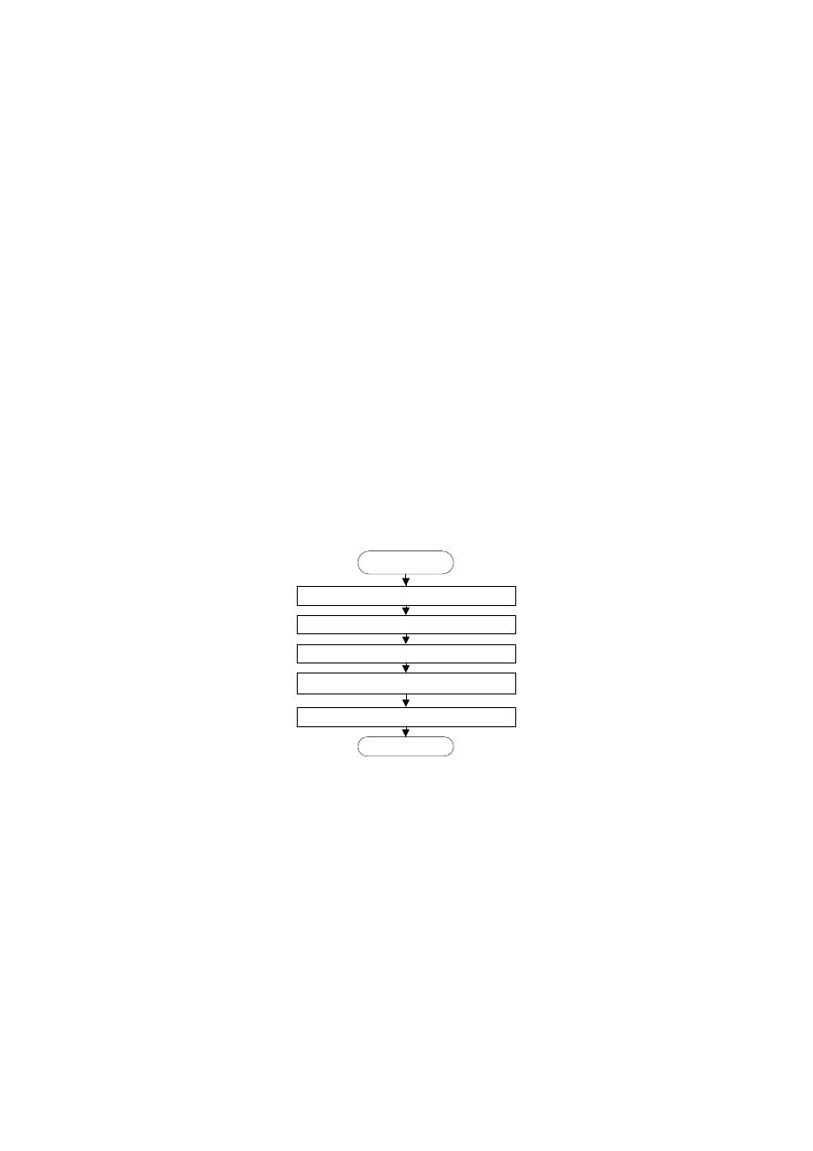
The developed design methodology using mock open tree topology consists in 5 basic sub-
processes which are shown in Figure 1 and explained below in this section. Note that the first and
last sub-processes in Figure 1 are exactly the same than in the former OPUS methodology.
However, there is an important variation in the middle steps of the algorithm since the new
approximation includes the use of IPL in order to design the tree structure network obtained from
the Sump Search step; instead of applying the optimal power use surface criterion and a subsequent
optimal flow distribution.
Sump Search or Tree Structure. This step is based on two fundamental principles: The first one
states that a WDS of minimum cost should convey the water to each of the demand nodes from the
water sources, through a single route. This is drawn from the fact that redundancy is hydraulically
inefficient, even though it favors reliability. Therefore, open WDSs could be a lot cheaper than
looped networks, reason why this sub-process intends to decompose the looped system into an open
tree-like structure (a spanning tree), in order to identify the nodes in the original model that
correspond to the sumps of the open network (i.e., nodes with a lower head than that of all of its
neighbors).
Start
Sump Search
Mock tree design using IPL
Addition of missing pipes
Minimum diameter to new pipes
Optimization
End
Figure 1: Mock open tree methodology BPMN diagram.
The second principle follows from the flow expression derived from the Darcy-Weisbach and
Colebrook-White equations. Leaving all the other parameters constant, the flow (
) presents a
relation approximately proportional with the diameter to a power of 2.6. Assuming a standard pipe
cost equation and replacing the diameter according to this proportion, the cost per length of a pipe
as a function of its design flow behaves as shown in Figure 2; which means that as the design flow
for a pipe increases, the marginal cost decreases.
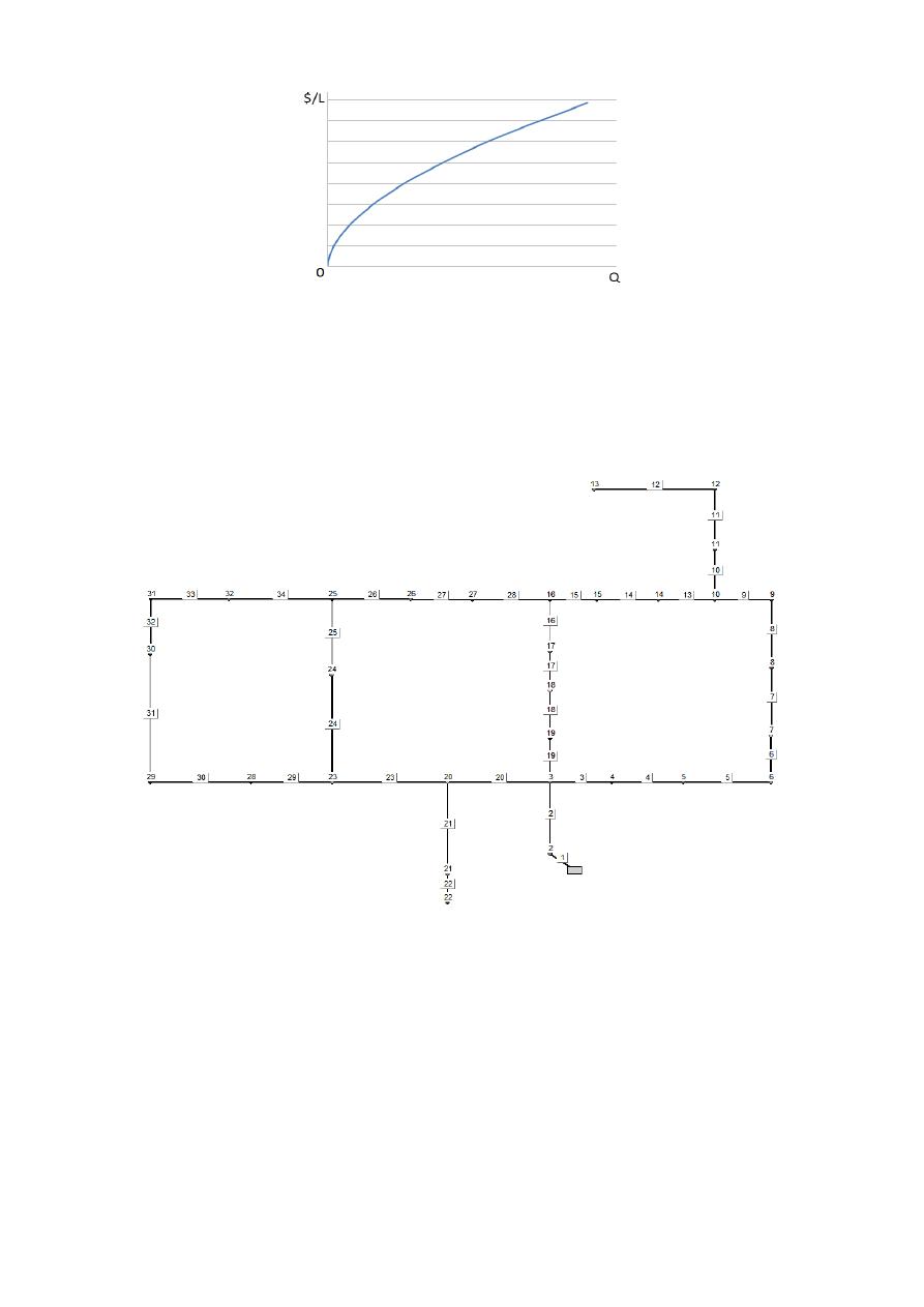
Figure 2: Schematic relation between pipe cost and flow.
From the abovementioned principles, an algorithm was designed in order to obtain the tree
structure, aggregating flow values in the least number of main routes possible. The open network is
set up starting from the water sources and then adding adjacent pipe-node pairs, one at a time. The
group of available pairs in each iteration conform the ‘search front’ and each of these pairs are
assigned a cost-benefit value (
), making up a recursive process.
Figure 3: Layout of the Hanoi WDS. The labels show pipe and nodal identification numbers.
For example, take the Hanoi benchmark WDS shown in Figure 3: Starting from the source, the first
pair to be added is the one consisting in pipe 1 and node 2 (<1, 2>). Then, the pair <2, 3> is added.
At this point the pairs <3, 4>, <19, 19> and <20, 20> can be selected. These constitute the search
front. Figure 3 shows the result for the entire execution of the sub-process, where the pipes
highlighted (solid black) constitute the corresponding tree structure.
The pair in the front with the higher cost-benefit value is selected to be part of the tree structure.
The cost-benefit function of a pair is calculated by computing the quotient between the demand of
the new node and the marginal cost of connecting it to the source: This entails the addition of the
total cost of the pair’s pipe to the cost difference of transporting the additional flow through all of
the upstream pipes. It is worth noting that these are not actual costs but proportional values drawn

from the relation shown in Figure 2. The construction of the tree using this cost-benefit function has
an O(NN
2
) time complexity, where NN is the number of nodes.
The cost-benefit function is used because it favours the creation of few main routes that transport
the largest portion of the total water volume. The process concludes when all of the system nodes
have been added to the tree structure and at the end the leaf nodes in the tree structure are assigned
the status of ‘sumps’.
Mock tree design using IPL. This sub-process focuses in designing the tree structure that resulted
from the previous step. The design is straightforward and is obtained applying the formulation
presented in (Hernández, 2012) which is implemented in the software Xpress IVE:
Sets
: Set that contains all the nodes.
: Set that contains all the commercially available diameters.
Decision variables
: Binary variable.
{
As it can be seen, de decision variable
can only take a value of 1 or 0; it will have a value of 1
if the model assigns a diameter of
to the section between node and node . Additionally, it is
necessary to define an auxiliary variable which contains the pressure of each node of the system.
: Auxiliary decision variable that defines the pressure in node .
Constraints of the problem
Constraint of
: Constraint that guarantees a HGL equal or greater than a minimum in every
node.
Constraint of HGL in downstream nodes: Constraint that guarantees that the HGL in node
downstream node
is equal to the HGL upstream minus the losses ( ) generated in the
pipeline section between node
and node provided that nodes and are linked.
∑
, |
where
corresponds to the hydraulic gradient line in node
, which is downstream node
. On the other hand
corresponds to the total head losses generated in the section
between nodes
and if a pipe of diameter is used.
corresponds to the decision variable. It is
worth noting that the values of
correspond to the total head losses obtained as parameters of
the problem, in the total head losses matrix.
Constraint of unique diameter in each section: This constraint guarantees that only one diameter is
assigned to each section of the system.

∑
, |
Objective function
∑ ∑ ∑
where
is the cost of using a diameter
in the section between node and node
.
corresponds to the decision variable. The objective is to minimize this function. The
constraints presented previously will be in charge of meeting the hydraulic requirements of
minimum pressure. It is worth noting that the values of
correspond to parameters of the
objective function, which are obtained from the cost matrix.
Knowing the flow demand in every node of the network, the minimum pressure required (
) and
the cost function; it is possible to calculate the cost matrix, total head losses matrix, connectivity
matrix and the minimum HGLs. From this and knowing the head in the reservoir, Xpress gives as a
result the minimum-cost design meeting the problem’s restrictions. This step contributes with as
many iterations as diameters are commercially available, due to the fact that in order to obtain the
head losses matrix it is necessary to assign the same diameter to all the pipes in the system and
execute a hydraulic simulation, this for every available diameter.
Addition of missing pipes. This step consists in adding to the tree structure the pipes that were
removed from the original network in the first step, in order to obtain again the latter. This is the
sub-process that allows the extension of the methodology using IPL to the design of looped
networks. Even though the network designed through IPL is an open structure, this is later
converted back again to a looped network to maintain the original topology.
Minimum diameter to new pipes. Due to the way in which the tree structure is generated, the open
network represents adequately the original network’s hydraulic behaviour, as long as the diameters
are the same for the common pipes. Namely, the pressure in the nodes will be the same in both
systems, since in theory the removed pipes don’t convey water because they link two sumps in
every case. This means that if the restriction of minimum pressure is fulfilled in the design of the
tree structure, it will be met as well in the looped network, despite the diameter assigned to the new
pipes. Given that the design obtained after the application of IPL is the optimum for the open
network, it is possible to just assign the minimum diameter to the rest of the pipes, so that the
capital cost of the network increases as least as possible; while the fulfilment of the discrete
diameter restriction is guaranteed.
This is valid for a single network, which in this case corresponds to a system with only one
reservoir. Reason why for networks with more than one water source it is necessary to make sure
that each node has a pressure at least equal to
. This is accomplished in the optimization step,
which is the final step of OPUS methodology, as well as the final step of the new approach
presented in this paper.
Optimization. This final sub-process has two main goals: The first one is to ensure every node has
a pressure higher than or equal to
; secondly, it seeks for possible cost reductions. Several
criteria could be used to establish the order in which pipes diameter values must be increased. It was
found that the pipes with larger unit head-loss difference between real and objective values should
be changed first. The process must continue until the whole system has acceptable pressures. The

second part executes a two-way sweep starting from the reservoirs going towards the sumps in the
direction of the flow, and then backwards: The reduction of each pipe’s diameter is considered
twice. If any of these changes entails a pressure deficit it must be reversed immediately, otherwise it
holds. To make sure minimum pressure is not being violated numerous hydraulic simulations are
required.
In first place, the diameter size of one pipe is increased iteratively while there are nodes with
pressure deficit. Thus, this sub-process requires the most number of iteration of the whole
methodology, being necessary to run a hydraulic simulation per pipe, for each single diameter
modification. This sole heuristic can be used alone to obtain sound designs, in spite of this, it is
strongly dependant on the initial pipe configuration.
RESULTS
The methodology methodology using mock open tree topology was used on three benchmark
systems: Hanoi, Balerma and Taichung.
Hanoi
The Hanoi network was first presented by Fujiwara and Khang (1990) and similarly to Two-Loop
network, it has become a well-known benchmark WDS. The head-loss equation commonly used is
Hazen-Williams with a
, the minimum pressure for the design scenario is 30 m and the
pipes’ costs can be calculated using a potential function of the diameter with a unit coefficient of
$1.1/m and an exponent of 1.5.
The Mock Tree methodology reached a cost of $6’163,754 after 119 iterations. Although this is not
the least cost reported, the number of hydraulic simulations needed to reach this result is three
orders of magnitude smaller than that of other approaches, as can be seen in Table 1. The pipe
diameter sizes in inches for this configuration are: 40, 40, 40, 40, 40, 40, 40, 40, 40, 30, 30, 24, 20,
16, 12, 12, 16, 20, 20, 40, 20, 12, 40, 30, 30, 20, 12, 12, 16, 16, 12, 12, 16 and 24 (these diameters
are shown in order of pipe identification number).
Table 1: Reported costs and number of iterations for the Hanoi WDS.
Algorithm
Cost (millions)
Number of iterations
Genetic Algorithm (Savic and Walters, 1997)
$6.073
1,000,000
Simulated annealing (Cunha and Sousa, 1999)
$6.056
53,000
Harmony search (Geem, 2002)
$6.056
200,000
Shuffled frog leaping (Eusuff and Lansey, 2003)
$6.073
26,987
Shuffled complex evolution (Liong & Atiquzzaman, 2004)
$6.220
25,402
Genetic Algorithm (Vairavamoorthy, 2005)
$6.056
18,300
Ant colony optimization (Zecchin et al., 2006)
$6.134
35,433
Genetic Algorithms (Reca & Martínez, 2006)
$6.081
50,000
Genetic Algorithms (Reca et al., 2007)
$6.173
26,457
Simulated annealing (Reca et al., 2007)
$6.333
26,457
Simulated annealing with tabu search (Reca et al., 2007)
$6.353
26,457
Local search with simulated annealing (Reca et al., 2007)
$6.308
26,457
Harmony search (Geem, 2006)
$6.081
27,721

Cross entropy (Perelman & Ostfeld, 2007)
$6.081
97,000
Scatter search (Lin et al., 2007)
$6.081
43,149
Modified GA 1 (Kadu, 2008)
$6.056
18,000
Modified GA 2 (Kadu, 2008)
$6.190
18,000
Particle swarm harmony search (Geem, 2009)
$6.081
17,980
Heuristic based approach (Mohan S. a., 2009)
$6.701
70
Differential evolution (Suribabu C. , 2010)
$6.081
48,724
Honey-bee mating optimization (Mohan S. a., 2010)
$6.117
15,955
Heuristic based approach (Suribabu C. , 2012)
$6.232
259
SOGH (Ochoa, 2009)
$6.337
94
OPUS (Saldarriaga, Páez, Cuero, & León, 2012)
$6.173
83
Mock Tree (this study)
$6.163
119
Extrapolating the cost function for a 50” diameter it would have a unit cost of $388.91/m. Taking
this into account, the total cost of the design obtained following the Mock Tree algorithm was of
only $5’414,077, with a total of 58 iterations. The diameter sizes in inches are: 40, 50, 40, 40, 40,
40, 30, 30, 30, 24, 24, 20, 16, 12, 12, 12, 16, 16, 20, 40, 16, 12, 30, 30, 30, 20, 12, 12, 16, 12, 12,
12, 16, and 20.
Balerma
Balerma corresponds to a WDS of an irrigation district in Almería, Spain. The pipe diameter sizes
commercially available for its design are manufactured exclusively in PVC, with an absolute
roughness coefficient of 0.0025 mm. The minimum pressure allowable is of 20 m and the pipes’
costs are calculated using a potential function, with a power of 2.06. Its topology is presented in
Figure 4.
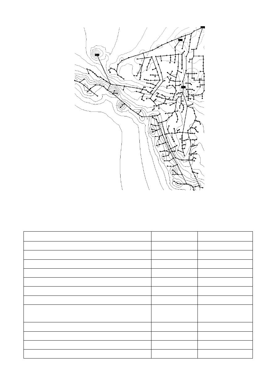
Figure 4: Topology of the Balerma network.
As a result of implementing the Mock Tree methodology on this network, a €2.148 millions discrete
design was found. Table 2 presents other reported costs and their respective number of iterations.
Table 2: Reported costs and number of iterations for the Balerma WDS.
Algorithm
Cost (
€
millions) Number of iterations
Genetic algorithm (Reca & Martínez, 2006)
2.302
10,000,000
Harmony search (Geem, 2006)
2.601
45,400
Harmony search (Geem, 2006)
2.018
10,000,000
Genetic algorithm (Reca et al., 2007)
3.738
45,400
Simulated annealing (Reca et al., 2007)
3.476
45,400
Simulated annealing with taboo search (Reca et al., 2007)
3.298
45,400
Local search with simulated annealing (Reca et al., 2007)
4.310
45,400
Hybrid discrete dynamically dimensioned search
(Tolson, 2009)
1,940
30,000,000
Harmony search with particle swarm (Geem, 2009)
2.633
45,400
SOGH (Ochoa, 2009)
2.100
1,779
Memetic algorithm (Baños, 2010)
3,120
45,400
Genetic heritage evolution by stochastic transmission
2,002
250,000

(Bolognesi, 2010)
Differential evolution (Zheng, 2012)
1,998
2,400,000
Self-adaptive differential evolution (Zheng, 2012)
1,983
1,300,000
OPUS (Saldarriaga, Páez, Cuero, & León, 2012)*
2.040
957
Mock Tree (this study)
2.148
826
*The result reported in the cited paper (€2.106 millions) has been recently improved.
Taichung
Taichung network was first presented by (Sung, Lin, Lin, & Liu, 2007) and it corresponds to a
WDS located in Taichung, Taiwan. The network’s topology consists of 20 nodes and 31 pipes
organized in 12 loops. For its design there are 13 pipe diameter sizes commercially available, which
costs are presented in Table 3. The head-loss equation used is Hazen-Williams with a roughness
coefficient (C) of 100 and the minimum pressure for the design scenario is 15 m. Its topology is
presented in Figure 5.
Table 3: Unit costs of Taichung network.
Diameter (mm)
Cost (NT Dollar m
-1
)
100
860
150
1160
200
1470
250
1700
300
2080
350
2640
400
3240
450
3810
500
4400
600
5580
700
8360
800
10400
900
12800
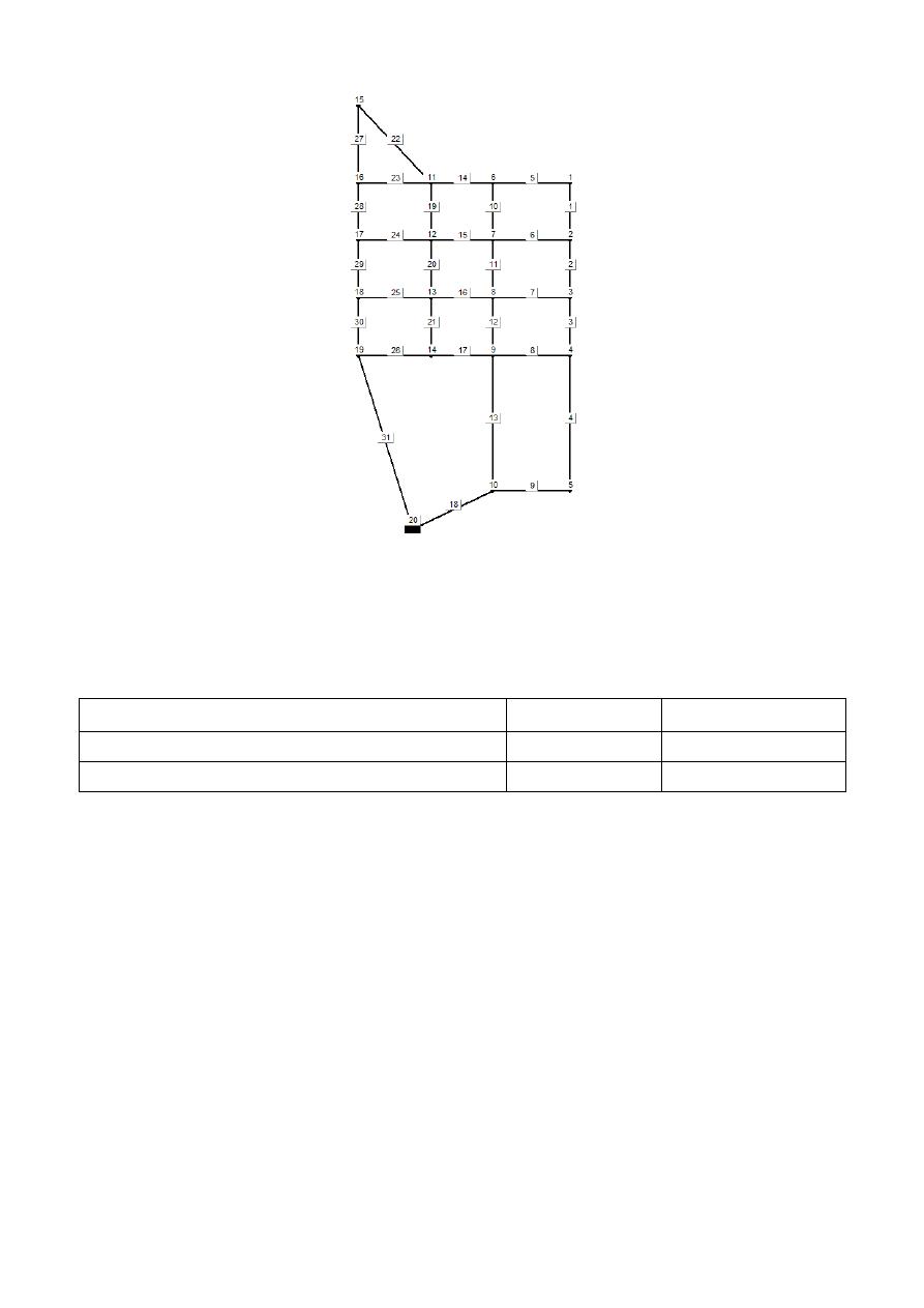
Figure 5: Topology of Taichung network. The labels show pipe and nodal identification numbers.
The Mock Tree methodology reached a cost of $8’774,900 after 48 iterations. The pipe diameter
sizes in millimetres for this configuration are: 250, 100, 150, 100, 100, 200, 100, 200, 150, 100,
250, 300, 350, 100, 100, 100, 100, 400, 150, 100, 100, 100, 100, 200, 100, 150, 100, 200, 250, 250,
and 300 (these diameters are shown in order of pipe identification number).
Table 4: Reported costs and number of iterations for the Taichung WDS.
Algorithm
Cost (
NT Dollar
)
Number of iterations
Tabu search (Sung, Lin, Lin, & Liu, 2007)
8,774,900
Not Available
Mock Tree (this study)
8,966,900
48
CONCLUSIONS
The WDS least-cost design methodology using mock open tree topology herein introduced,
considers hydraulic criteria to transform a looped network into an open structure, which is later
designed using IPL. This approach differentiates it from the OPUS methodology which first
produces a continuous design that is then transformed into a discrete design, through different
approximation criteria. Even though these two methodologies have different approximations, they
have in common the use of hydraulic principles, unlike metaheuristic algorithms that explore the
solution space without considering this kind of criteria.
The methodology significantly reduces the number of iterations and keeps the constructive costs of
the network very close to the minimum. In the case of Hanoi the difference results of only 2% with
respect to the lowest cost reported in the literature and with a number of iterations four orders of
magnitude below.

This methodology clearly proves that considering hydraulic bases together with IPL principles
allows the optimization of WDS design to reduce significantly the number of iterations required.
The results here found are significantly close to the records, and a little improvement of these would
require a really big effort. For this, it is recommended to use this methodology as the basis for new
ones but it is not worth it to invest efforts in refining it.
REFERENCES
Alperovits, E., and Shamir, U. (1977) Design of optimal water distribution systems. Water
Resources Research, Vol.13, No.6, pp. 885-900.
Baños, C. G. (2010). A memetic algorithm applied to the design of water distribution networks.
Applied Soft Computing, 261-266.
Bolognesi, A. e. (2010). Genetic Heritage Evolution by Stochastic Transmission in the optimal
design of water distribution networks. Advances in Engineering Software, 792-801.
Cunha, M. a. (1999). Water distribution network design optimization: Simulated annealing
approach. J. Water Resour. Plan. Manage. , 215-221.
Eusuff, M. a. (2003). Optimization of water distribution network design using the shuffled frog
leaping algorithm. J. Water Resour. Plan. Manage. , 210-225.
Fujiwara, O. and Khang, D. (1990). A two phase decomposition methods for optimal design of
looped water distribution networks. Water Resources Research, Vol.26, No. 4, pp. 539-549.
Geem, Z. K. (2002). Harmony search optimization: Application to pipe network design. Int. J.
Model. Simulat. , 125-133.
Geem, Z. K. (2006). Optimal cost design of water distribution networks using harmony search.
Engineering Optimization, Vol.38, No.3, pp. 259-277.
Geem, Z. K. (2009). Particle-swarm harmony search for water network design. Engineering
Optimization, Vol.41, No.4, pp. 297-311.
Hernández, D. (2012). Diseño optimizado de submódulos de sistemas de riego localizado a alta
frecuencia. Bogotá, DC: Universidad de los Andes.
Kadu, M. R. (2008). Optimal design of water networks using a modified genetic algorithm with
reduction in search space. J. Water Resour. Plan. Manage. , 147-160.
Lin, M., Liu, G. and Chu, C., (2007) Scatter search heuristic for least-cost design of water
distribution networks, Engineering Optimization, Vol.39, No.7, pp. 857-876.
Liong, S. and Atiquzzaman, M. (2004) Optimal design of water distribution network using shuffled
complex evolution. Journal of the Institution of Engineers, Vol.44, No.1, pp. 93-107.
Mohan, S. a. (2010). Optimal water distribution network design with Honey-Bee mating
optimization. J. Water Resour. Plan. Manage., 117-126.
Mohan, S. a. (2009). Water distribution network design using heuristics-based algorithm. J.
Comput.Civ. Eng., 249-257.
Ochoa, S. (2009). Optimal design of water distribution systems based on the optimal hydraulic
gradient surface concept. MSc Thesis, dept. of Civil and Environmental Engineering,
Universidad de los Andes, Bogotá, Col. (In Spanish).
Perelman, L. and Ostfeld, A. (2007). An adaptive heuristic cross entropy algorithm for optimal
design of water distribution systems. Engineering Optimization, Vol.39, No.4, pp. 413-428.
Reca, J. and Martínez, J. (2006). Genetic algorithms for the design of looped irrigation water
distribution networks. Water Resources Research, Vol.44, W05416.
Reca, J., Martínez, J., Gil, C. and Baños, R. (2007). Application of several meta-heuristic
techniques to the optimization of real looped water distribution networks. Water Resources
Management, Vol.22, No.10, pp. 1367-1379.
Saldarriaga, J. (1998 and 2007). Hidráulica de Tuberías. Abastecimiento de Agua, Redes, Riegos.
Ed. Alfaomega. Ed. Uniandes. ISBN: 978-958-682-680-8.

Saldarriaga, J., Takahashi, S., Hernández, F. and Escovar, M. (2011). Predetermining pressure
surfaces in water distribution system design. In Proceedings of the World Environmental and
Water Resources Congress 2011, ASCE.
Saldarriaga, J., Páez, D., Cuero, P., & León, N. (2012). Optimal power use surface for design of
water distribution systems. XIV Water Distribution Systems Analysis Conference. Tucson,
Arizona, USA.
Savic, D. and Walters, G. (1997). Genetic algorithms for least cost design of water distribution
networks. J. Water Resour. Plan. Manage., 67-77.
Sung, Y.-H., Lin, M.-D., Lin, Y.-H. L., & Liu, Y.-L. (2007). Tabu search solution of water
distribution network optimization. Journal of Environmental Engineering and Management,
177-187.
Suribabu, C. a. (2006). Design of water distribution networks using particle swarm optimization.
Urban Water Journal, 111-120.
Suribabu, C. (2010). Differential evolution algorithm for optimal design of water distribution
networks. J. of Hydroinf., 66-82.
Suribabu, C. (2012). Heuristic Based Pipe Dimensioning Model for Water Distribution Networks.
Journal of Pipeline Systems Engineering and Practice, 45 p.
Takahashi, S., Saldarriaga, S., Hernández, F., Díaz, D. and Ochoa, S. (2010). An energy
methodology for the design of water distribution systems. In Proceedings of the World
Environmental and Water Resources Congress 2010, ASCE.
Tolson, B. A. (2009). Hybrid discrete dynamically dimensioned search (HD-DDS) algorithm for
water distribution system design optimization. Water Resources Research, 45 p.
Vairavamoorthy, K. a. (2005). Pipe index vector: A method to improve genetic-algorithm-based
pipe optimization. J. Hydraul. Eng., 1117-1125.
Villalba, G. (2004). Optimal combinatory algorithms applied to the design of water distribution
systems. MSc Thesis, dept. of Systems and Computation Engineering, Universidad de los
Andes.
Wu, I. (1975). Design of drip irrigation main lines. Journal of Irrigation and Drainage Division,
Vol.101, No.4, pp. 265-278.
Wu, Z. and Simpson, A. (2001). Competent genetic evolutionary optimization of water distribution
systems. Journal of computing in civil engineering. Vol.15, No.2, 2001, pp. 89-101.
Yates, D., Templeman, A. and Boffey, T. (1984). The computational complexity of the problem of
determining least capital cost designs for water supply networks. Engineering Optimization,
Vol. 7, No.2, pp. 142-155.
Zecchin, A., Simpson, A., Maier, H., Leonard, M., Roberts, A., and Berrisfors, M. (2006)
Application of two ant colony optimization algorithms to water distribution system
optimization. Mathematical and Computer Modeling, Vol.44, No. 5-6, pp. 451-468.
Zheng, F. e. (2012). A Self
‐Adaptive Differential Evolution Algorithm Applied to Water
Distribution System Optimization. Journal of Computing in Civil Engineering, 45 p.
