
water
Article
Use of Energy-Based Domain Knowledge as Feedback
to Evolutionary Algorithms for the Optimization of
Water Distribution Networks
Diego Páez
1
, Camilo Salcedo
2
, Alexander Garzón
3
, María Alejandra González
3
and
Juan Saldarriaga
4,
*
1
Department of Civil Engineering, Queen’s University, Kingston, ON K7L 3N6, Canada;
da.paez270@gmail.com
2
Department of Civil & Architectural Engineering & Mechanics, University of Arizona, Tucson, AZ 85721,
USA; csalcedo@email.arizona.edu
3
Water Supply and Sewer Systems Research Center (CIACUA), Universidad de los Andes, Bogotá 111711,
Colombia; ja.garzon11@uniandes.edu.co (A.G.); ma.gonzalezm1@uniandes.edu.co (M.A.G.)
4
Department of Civil and Environmental Engineering, Universidad de los Andes, Bogotá 111711, Colombia
*
Correspondence: jsaldarr@uniandes.edu.co; Tel.:
+57-1-339-49-49 (ext. 2805)
Received: 8 July 2020; Accepted: 28 October 2020; Published: 4 November 2020
Abstract:
The optimization of water distribution networks (WDN) has evolved, requiring approaches
that seek to reduce capital costs and maximize the reliability of the system simultaneously.
Hence, several evolutionary algorithms, such as the non-dominated sorting-based multi-objective
evolutionary algorithm (NSGA-II), have been widely used despite the high computational costs
required to achieve an acceptable solution. Alternatively, energy-based methods have been used to
reach near-optimal solutions with reduced computational requirements. This paper presents a method
to combine the domain knowledge given by energy-based methods with an evolutionary algorithm,
in a way that improves the convergence rate and reduces the overall computational requirements to
find near-optimal Pareto fronts (PFs). This method is divided into three steps: parameters calibration,
preprocessing of the optimal power use surface (OPUS) results, and periodic feedback using OPUS in
NSGA II. The method was tested in four benchmark networks with di
fferent characteristics, seeking
to minimize the costs of the WDN and maximizing its reliability. Then the results were compared
with a generic implementation of NSGA-II, and the performance and quality of the solutions were
evaluated using two metrics: hypervolume (HV) and modified inverted generational distance (IGD
+).
The results showed that the feedback procedure increases the e
fficiency of the algorithm, particularly
the first time the algorithm is retrofitted.
Keywords:
multi-objective evolutionary algorithm; NSGA-II; optimal power use surface (OPUS);
hypervolume; IGD
+; domain knowledge; hot start
1. Introduction
Water is the source and sustenance of life, as it has unique properties that make it essential for all
living things. However, there are still many people who do not have access to drinking water due
to the investment and maintenance costs of water distribution systems (WDS). This problem is very
common in developing countries. For this reason, one of the most common optimization problems
is the minimum cost design of WDS, which serves to determine the diameter of the network pipes
satisfying hydraulic conditions. Moreover, in recent years the optimal design of WDS has changed
because a second objective was included in the optimization problem. For solving the new design
Water 2020, 12, 3101; doi:10.3390
/w12113101
www.mdpi.com
/journal/water

Water 2020, 12, 3101
2 of 23
problem, it was necessary to change from single-objective formulations to bi-objective formulations to
obtain a Pareto front (PF) that includes a set of di
fferent optimal solutions.
It has been found that the optimal design in WDS belongs to the category of non-deterministic
polynomial time-hard problems (NP-hard problems) [
1
], because of the polynomial given by the
equations for energy conservation and the presence of discrete variables. This implies that finding
an optimal solution using deterministic and exhaustive methods becomes practically impossible for
real-sized networks. However, approximate methods can be implemented to provide near-optimal
solutions. Di
fferent approaches have been made, including linear and nonlinear programming
approximations [
2
], but metaheuristic algorithms replaced these approaches due to their easy
applicability, a greater analysis of the solution space, and their ability to include the constraints
given by the discrete-sized diameters. Some of the most common metaheuristic algorithms are genetic
algorithms [
3
], simulating annealing [
4
], harmony search [
5
], shu
ffled frog leaping algorithm [
6
],
and particle swarm optimization [
7
].
Another alternative, less explored due to the development of metaheuristic methods, was to
compute and analyze the optimal design for simple networks and determine some patterns in the
results and the hydraulic principles that generate them, to apply them in more complex systems. One of
the first researchers to carry out this type of research was Wu [
8
], who developed an optimal criterion
for the design of drip irrigation systems with uniform demands and varied topography. After analyzing
many scenarios, he concluded that the optimal design was obtained by the hydraulic gradient line
(HGL) followed a parabolic shape with a sag of 15% with respect to a straight HGL. In 1983, Featherson
and El-Jumaily [
9
] suggested applying Wu’s criterion to looped networks. This procedure assumes an
initial set of diameters for the pipes, and then adjusting them to fit an ideal hydraulic gradient line.
Subsequently, Takahashi et al. [
10
] introduced the optimal power use surface (OPUS) methodology for
looped networks, based on the optimal HGL criterion and other hydraulic criteria. In 2020, Saldarriaga
et al. [
11
] implemented the OPUS methodology in four di
fferent benchmark networks to compare the
e
fficiency of applying hydraulic principles with other metaheuristics algorithms. They concluded that
OPUS is a suitable method that can be easily applied to real networks, minimizing construction costs
in a lower number of iterations than other methodologies.
Nevertheless, the design of drinking water distribution systems cannot be based exclusively
on the least-cost criterion, since other variables are also crucial for determining the optimal design
solution, such as network resilience and reliability or water quality. For this reason, in the last two
decades, multi-objective evolutionary algorithms (MOEAs) have been used to e
fficiently explore the
solution space finding a suitable approximation of the PF. Deb et al. [
12
] proposed a non-dominated
sorting-based multi-objective evolutionary algorithm (NSGA-II), which has been used on multiple
occasions for the optimal design of WDS. For example, Farmani et al. [
13
] used the NSGA-II to minimize
cost and number of nodes with head deficiency in a real benchmark network. Similarly, Prasad and
Park [
14
] used the same methodology for designing a WDS, with the objectives of minimizing
costs and maximizing the network resilience, obtaining a set of Pareto optimal solutions for two
benchmark networks.
As stated before, reliability has become an important objective to guide the optimal design of
water networks besides the cost. Hence, regarding the reliability of a WDS, it can be divided into
two categories: mechanical and hydraulic. Mechanical reliability refers to the degree to which the
WDS can continue to provide adequate levels of service during an atypical event [
15
]. One of the
most widely used indicators of mechanical reliability for the analysis of WDS is the entropy reliability
indicator (ERI) [
16
]. On the other hand, hydraulic reliability refers to the tolerance of the network for
changes over time, such as demand variations [
15
]. Some of the most used indexes for measuring
hydraulic reliability are Todini’s resilience index (RI), network resilience index (NRI), minimum
surplus head (MSH), total surplus head (TSH), and modified resilience index (MRI)[
16
]. To determine
which indicator best describes the reliability of the network, multiple authors have made comparisons
between di
fferent indexes. Raad et al. [
17
] compared four reliability measures, three commonly used

Water 2020, 12, 3101
3 of 23
(RI, NRI, and flow entropy) and a new mixed reliability measure, by applying them in three WDS
benchmarks. In conclusion, the RI showed the best performance under a demand variation, while
NRI and the mixed reliability measure performed better after pipe failure conditions. Creaco et al. [
18
]
compared entropy and two reliability indexes (NRI and RI) in two case studies with di
fferent topologies
to determine which indicator best describes the reliability of a WDN. As a result, they obtained that
the index that best describes the reliability of a simple and complex network is NRI. However, it is
important to clarify that these indexes are not a measure of network resilience in some cases. Thus,
Zhan et al. [
19
] compared four resilience-related indexes, that included Todini’s resilience index and
three direct performance indicators for the optimization of three WDS networks. The results showed
the existence of high correlations between the four resilience-related indicators, which served to
improve the system resilience measure using any other index. However, each one of the indicators
showed both advantages and disadvantages. For instance, Todini’s resilience index showed a high
correlation with the direct resilience indicator in the networks without a water tank, but this index
should not be used in networks with tanks because the correlation is weaker for those networks.
Hybrid algorithms have recently been developed to extend search e
fficiency within the solution
space. Raad et al. [
20
] applied a meta-algorithm called AMALGAM and the jumping-gene genetic
algorithm (NSGA-II-JG) to the design of WDS. The objectives of the design were to minimize cost
and maximize a resilience measure. By implementing all the methods in one case study, AMALGAM
obtained the best-quality results in comparison with NSGA-II and NSGA-II-JG. To determine the
e
fficiency of different MOEAs, Wang et al. [
21
] compared five di
fferent multi-objective evolutionary
algorithms in twelve benchmark networks. The MOEAs tested include two modern hybrid MOEAs:
ε
-MOEA and ε-NSGA-III, and three frequently used MOEAs: NSGA-II, AMALGAM, and Borg MOEA.
They concluded that the NSGA-II is one of the best MOEAs, because it showed the best achievements
in all the benchmarks. Furthermore, from the implemented MOEAs, Wang et al. [
21
] determined the
best Pareto front for each benchmark network. Most recently, Cunha and Marques [
22
] developed
a new multi-objective algorithm based on simulated annealing, including the new generation and
re-annealing procedures (MOSA-GR) to minimize the total cost of pipes and maximize the network
resilience for the design of WDS. By using this algorithm, there was an improvement in the convergence
and diversity of the solutions found in the PF. Initially, it implements a new process for the generation of
individuals. After these solutions are obtained, a new stage begins where the re-annealing procedure is
implemented to improve the non-dominated individuals found. As a result, MOSA-GR improved the
PF obtained by the MOEAs; it generated new solutions that redefine some parts of the best-known front
and extended the established boundaries for nine benchmark networks (New York, Blacksburg, Hanoi,
GoYang, Fossolo, Pescara, Modena, Balerma and the Exeter network). However, for the other three
study cases (two-reservoir, two-toops and BakRyan networks) classified as small networks, the true PF
were established by Wang et al. [
21
]. Given the size of their search space, a complete enumeration can
be performed, reaching the true PF. Hence, no further improvements are possible to reach [
22
].
On the other hand, new hybrid algorithms have been developed from the combination of two
methodologies. The first to propose a low-level hybrid procedure were Creaco and Franchini [
23
], who
combined linear programming and the multiple objective genetic algorithm NSGA-II for the design of
a group of branched networks. The new algorithm showed benefits in terms of computational and
numerical e
fficiency. More recently, Yazdi et al. [
24
] developed a hybrid algorithm called non-dominated
sorting harmony search di
fferential evolution (NSHSDE), which is the combination of differential
evolution (DE) and harmony search (HS). This new method was compared to NSGA-II, strength Pareto
evolutionary algorithm II (SPEA-II), and MOEA
/D. They obtained that NSHSDE provided better
optimal solutions than the other MOEAs used.
The application of evolutionary algorithms (EA) to the WDS optimization problem may require
high computational costs, due to their complexity. As a solution in recent years, engineering knowledge
has been implemented to decrease the size of the initial population or the search space to obtain good
results of the PF in less computational time. Keedwell and Khu [
25
] implemented a cellular automata

Water 2020, 12, 3101
4 of 23
approach for the design of WDS. In the generation of the initial population, they applied three rules
which related the head at each node and the diameter of the pipes. For example, if the junction had a
head deficit, it was necessary to increment the diameters of the pipes connected to that node.
On the other hand, Kang and Lansey [
26
] used engineering judgment to improve the results of
genetic algorithms when applying it to the design of WDN. To determine the initial population of
individuals, they used engineering knowledge about optimal flow velocities in WDNs. Bi et al. [
27
]
developed a high-quality initial population by using the multi-objective prescreened heuristic sampling
method (MOPHSM) for the optimal design of WDS. The MOPHSM assigns the diameter of the
pipe depending on its distance to the source of water and the optimal flow velocity. More recently,
Liu et al. [
28
] determined the first generation of individuals of GA, using a new methodology called
head-loss-based design preconditioner (HDP). This method calculates the initial diameter of the pipes by
analyzing head losses from the network. HDP was implemented in three WDS networks and compared
with prescreened heuristic sampling method (PHSM) made by Bi et al. [
29
]. Finally, the results showed
a better performance for HDP method in terms of computational cost and quality solution.
In order to evaluate the quality of the PFs generated by using MOEAs, di
fferent metrics are used.
Among the most used are hypervolume index (HV), generational distance (GD), spacing (S), coverage
set (CS), inverted generational distance (IGD
+), and diversity comparison indicator (DCI). Bi et al. [
27
]
used three run-time performance metrics to understand the speed at which the proposed multi-objective
algorithm generated the PF for the optimization of cost and resilience of a WDS. The metrics used were
hypervolume, generational distance, and extent of the front. Similarly, Yazdi et al. [
24
] analyzed four
di
fferent metrics to solve the same problem, but they used a hybrid algorithm that combines the global
search structure of di
fferential evolution (DE) with the local search skills provided by harmony search
(HS). Based on previous studies, the hypervolume (HV) and modified inverted generational distance
(IGD
+) were used in this research to evaluate the performance of the proposed algorithm, due to their
advantages in respect to the properties of the PFs that they take into account, such as uniformity and
convergence, among others.
This paper aims to present a methodology for the optimal design of water distribution networks
(WDN), minimizing the capital cost of the system and maximizing its reliability. However, the proposed
methodology seeks to emphasize the improvement of the convergence rate of the NSGA-II algorithm
by using constant feedback from an optimal design reached using an energy-based method, in this case,
the optimal power use surface (OPUS) [
10
]. First, a description of the optimization problem is made in
which the objectives to maximize and minimize are described, including the corresponding constraints.
Then, a description of OPUS and NSGA-II algorithms is presented as an introduction to the bases for
the feedback procedure. Both NSGA-II and the proposed algorithm were tested in four benchmark
networks (Hanoi, Fossolo, Modena, and Balerma), reaching an approximation to the optimal PF used as
a reference [
21
]. Afterward, the performance of the algorithms was evaluated using the hypervolume
(HV) and the modified inverted generational distance (IGD
+). Finally, the results are shown and
analyzed, evidencing that in three of the tested cases, the proposed algorithm reached a good-quality
solution with increased e
fficiency, delivering better performance for large realistic networks. Hence,
using an energy-based method to feedback an evolutionary algorithm was successfully proven as an
e
fficient way to improve the convergence rate for these widely used methods.
2. Optimization Problem
The optimal design problem in WDSs is addressed as a multi-objective approach that seeks to
(1) minimize the constructive costs of the network, and (2) maximize a reliability-based index of the
network. In this research, the reliability of the network is assessed using a performance measurement
known as the network resilience index (NRI), which is founded in the Todini’s resilience index [
30
].
However, this index incorporates both the e
ffects of surplus power at the nodes and reliable loops in
the system, considering the uniformity in the diameters connected to a node [
14
]. The two objectives
used in this approach can be described as follows:

Water 2020, 12, 3101
5 of 23
Minimize Cost:
C
Total
=
np
X
i=1
U
c
·D
i
·L
i
(1)
Maximize NRI
NRI
=
P
m
j=1
U
j
DM
j
H
j
− H
∗
j
P
R
r=1
q
r
H
R
r
− P
m
j=1
DM
j
H
∗
j
+
z
j
; U
j
=
P
p∈M
D
p
M
j
·max
p
M
j
n
D
p
o
(2)
where C
Total
is the total network cost, which includes the material and construction costs; np is the total
number of pipes; D
i
and L
i
stand for the diameter and the length of the i-th pipe; and U
c
corresponds
to the unit pipe cost for the D
i
diameter. Regarding the network resilience index, U
j
represents an
indicator for diameter uniformity; H
j
and DM
j
are the pressure head and the nodal demands for the j-th
node; H
j
*
is the minimum allowable pressure head at the j-th node; q
r
and H
r
R
are the total demands
and total heads provided by the supply source, respectively; z
j
is the elevation of the j-th node; D
p
is
the diameter that belongs to a set M
j
, which represents all the pipes that are connected to the j-th node,
and
|M
j
| is the cardinality of M
j
.
The proposed optimization problem is subject to several constraints. In the first place, for service
purposes, a minimum pressure is required in the demand nodes, whereas to avoid operational
inconveniences, maximum pressure is required, as well as a maximum velocity in the pipes of the
system. Secondly, the hydraulic constraints of the network must be met, which include mass and
energy conservation in nodes and pipes, respectively, and finally, the selection of a discrete set of
diameters for the pipes. While the hydraulic constraints are met by using a hydraulic simulator, such as
EPANET, the service constraints were handled by using cost-to-completion static penalty functions
incorporated into the algorithm and activated in case the constraints were not met.
The pressure constraints were handled by penalizing the objective functions according to the
pressure penalty shown in Equation (3), which considers both minimum and maximum pressures.
In this expression, PS
i
stands for the maximum pressure surplus in the network, calculated as
the di
fference between the pressure at each demand node and the maximum allowable pressure
correspondingly; PS
max
corresponds to the maximum allowable pressure surplus within the network;
P
min
stands for the minimum pressure required at each junction and NMP is the network minimum
pressure registered for each individual.
Pressure Penalty
=
max
(
PS
i
PS
max
,
P
min
− NMP
P
min
!)
∗ P
Ratio
(3)
Similarly, the velocity constraint was ensured by using the velocity penalty shown in Equation (4).
In this expression, V
max
corresponds to the maximum velocity allowable in the pipes, and NMV stands
for the network’s maximum velocity registered for each individual. This penalty function will be used
only for the case studies that established a maximum velocity constraint.
Velocity Penalty
=
max
0,
V
max
− NMV
V
max
∗ P
Ratio
(4)
Finally, the parameter P
Ratio
used in both penalty functions establishes the magnitude of the
penalization for the pressure and velocity penalties. This value ranges between 1E06 and 1E09,
depending on the tested network, and it was calibrated with the other parameters of the algorithms,
as described later in this paper.

Water 2020, 12, 3101
6 of 23
3. Methodology for the Optimal Design of Water Distribution Systems
3.1. OPUS
OPUS is an optimized WDS design methodology based on the HGL criterion introduced by
Wu [
8
] and other hydraulic criteria. In order to understand the energy flow of the network, the OPUS
methodology is implemented in six steps. First, OPUS—a spanning tree structure is identified for
the looped network based on two basic hydraulic principles: (1) the water demand of each node
must be supplied from the water sources using a single route for the least-cost WDS case; and (2) the
determination of an equation that relates the pipe diameter and its cost per length unit [
11
]. The first
hydraulic principle is based on the fact that redundancy is hydraulically ine
fficient, even though
it increases reliability. For this reason, this process aims to decompose the looped network into a
spanning-tree because looped systems can be more expensive than open networks [
10
]. From this
process, it is possible to identify the nodes that can be considered as sumps (i.e., nodes with a lower head
than those that are nearby) [
10
]. The other principle uses the Hazen–Williams equation to determine
that as the design flow rate of a pipe increases, the marginal cost decreases [
11
]. The spanning-tree
begins to be built from the water source and increases by adding adjacent nodes, always ensuring that
the search front reaches the highest cost-benefit value. This process ends until all the systems nodes
have been added to the spanning tree [
11
].
The second step, optimal power surface, is to determine the head-losses of each pipe by assigning
a target HGL for every node [
11
]. First, a minimum permissible pressure value is assigned to all
sump’s nodes. Then, the HGL is calculated using the topological distance from each node to the
reservoir and its head. It is possible to determine a series of parabolic functions that serve to find
objective head values for each node using the topological distances and the head of each source and
sump [
10
]. The methodology proposed by Ochoa [
31
] was used to estimate the optimal sag value.
This value depended on the ratio between flow demands and pipe length, the cost function, and the
demand distribution. The sag value should be calculated at each intersection; hence, the flow on
each downstream route must be weighted [
32
]. For avoiding the assignation of head values that do
not meet the pressure demand, nodes with high elevations should be analyzed. Once this process is
finished, the optimal power use surface must be formed since all the nodes are assigned an objective
head value [
10
].
The third step, known as optimal flow distribution, consisted of finding a single flow distribution
in the network that describes the optimal power use surface calculated in the previous step, ensuring
the mass conservation at each node. The optimal flow distribution is calculated by dividing the flow
demand into the upstream pipes, starting from the sumps. Saldarriaga et al. [
32
] created three criteria
for this procedure: (1) uniform distribution, where all pipes have the same flow, therefore the flow
demand of each node is divided into the number of upstream pipes connected to it; (2) proportional
distribution, where the flow is distributed proportionally to H
/L
2
, where L is the length of the pipes
and H its head losses; and (3) all-in-one distribution, where all pipes are assigned with the design flow
that corresponds to the minimum diameter available. The pipe with the highest value of hydraulic
favorability is assigned with the residual flow when design with the minimum diameter is insu
fficient
to transport the total flow demand [
11
].
Once the head of each node and the flow of every pipe are defined, the method calculates the
continuous diameter using the Hazen–Williams or Darcy–Weisbach equations. After calculating the
diameters, the method rounds the continuous values to discrete values found on the commercial
pipeline list [
11
]. This approach can be made in multiple ways; however, it was found that the best
results are obtained by approximating to the nearest flow. This is done by raising the continuous
diameter values to a power of 2.6 and round them [
32
]. The last process of OPUS ensures all nodes have
a pressure higher than the minimum value and reduce the diameters of the pipe, without violating any
restrictions, to decrease capital costs.

Water 2020, 12, 3101
7 of 23
3.2. NSGA-II
One of the most widely used multi-objective evolutionary algorithms in engineering optimization
problems is NSGA-II, developed by Deb [
12
]. For the design of WDS, it has been used to determine
the diameter of the pipes with the objectives of minimizing costs and maximizing a measure of
reliability [
21
]. The procedure of the NSGA-II is as follows: first, the algorithm generates a random
population between the upper and lower boundaries specified. Then, the individuals are sorted
according to non-domination and crowding distance. The elements of the population are selected by
the tournament method to create a mating pool with the best individuals. Those selected parents create
new individuals by crossover and mutations. Once these processes have been finished, the population
is twice as large as the original, in order to select the best individuals of these new population the
process of rank and crowding distance must be done again.
In this research, the algorithm has been used to design WDS minimizing cost and maximizing a
reliability surrogate measure, such as the NRI [
21
] by choosing the decision variables as the diameters
of each pipe, allowing them to take values from an available diameters list. Finally, NSGA-II was
implemented in this research because it is widely used for the design of WDS; however, any other
multi-objective evolutionary algorithm could be used instead.
3.3. NSGA-II with Intermittent Feedback from Energy Based Methods
The proposed method (OPUS-NSGA-II) includes the domain knowledge acquired by using OPUS
in the NSGA-II metaheuristic. It is divided into three steps as follows: (1) calibration process of the
parameters of the tested algorithms; (2) preprocessing of OPUS results; and (3) an intermittent feedback
to NSGA-II. These steps are described as follows.
3.3.1. Calibration Process
The calibration process performed in this research consisted of testing di
fferent values of the
parameters within the recommended ranges and searching to determine a set of parameters that could
better approximate the best-known Pareto front for each network.
An optimal set of parameters could be determined by the implementation of systematic approaches,
such as optimization. However, these procedures were not applied, given that the proposed
methodology sought to provide an improvement in the e
fficiency of the NSGA-II algorithm rather than
the achievement of better solutions than the reported. Hence, the set of parameters determined in this
procedure were su
fficient to establish a baseline for the comparison between the proposed algorithm
and NSGA-II by itself.
In relation with the NSGA-II algorithm, the following seven parameters were considered:
population size, number of generations, the crossover distribution index and the crossover probability
derived from using simulated binary crossover (SBX), the mutation distribution index and mutation
probability derived from the use of polynomial mutation (PM) and finally the P
Ratio
for both the pressure
and velocity penalty functions. Then, concerning the proposed methodology, the feedback frequency
was calibrated. Additionally, every network was tested with a di
fferent combination of parameters.
The population size and the number of generations for the study cases varied between (500, 4000)
and (500, 5000), respectively, according to the network size. As stated in previous studies, these
parameters have a high impact on the computational e
ffectiveness of the algorithm. Hence, enough
individuals may avoid a crowded population, while a better convergence can be ensured by performing
a larger number of generations [
33
].
The crossover distribution index considered values that range between 2 and 5, where using greater
values ensures fewer variations from parent chromosomes [
34
]. On the other hand, the mutation
distribution index typically ranges between 20 and 100, where greater values also ensure fewer
variations from parent chromosomes [
35
]. Regarding these operators, the probability of crossover
and the probability of mutation remained constant and equal to 0.9 and 0.1, respectively, for all the
Water 2020, 12, 3101
8 of 23
simulations performed. These values were fixed for all networks, given their minor impact on the
behavior of the NSGA-II algorithm, as previous studies have demonstrated [
33
].
For each parameter, the chosen values were selected after a visual inspection in which the
convergence to the optimal PF, the spread and distribution of the resulting PFs were the desirable
properties. Even though this was not an exhaustive search over the entire parameter space, it covered
di
fferent values within the ranges, and it allowed the definition of a robust NSGA II for every tested
WDS. Moreover, the set of parameters determined by the procedure described above was used in both
NSGA-II and the proposed algorithm.
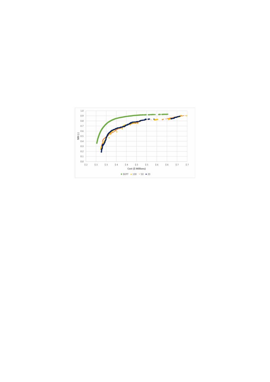
As an example, the comparison between di
fferent tested values for the mutation distribution
index for Modena after 500 generations is shown in Figure
1
.
Figure 1.
Comparison between tested values for the mutation distribution index after 500 generations
in Modena. BKPF
= Best-Known Pareto Front; NRI = network resilience index.
Regarding the proposed algorithm, the parameter m describes the frequency in which feedback
from OPUS is given to NSGA-II, as described in the next sections. For determining the corresponding
value for the parameter m at each case study, values between 1 and 100 were tested. This analysis was
performed after the other parameters were calibrated, and it sought to determine the best possible
values for the parameter to enhance the performance of NSGA-II by the retrofitting process with OPUS.
As a result, the e
ffect of this enhancement could be assessed by comparing both algorithms.
After the described procedure was performed, the recommended feedback frequency m was
established to be between 5 and 50 generations.
Finally, based on the previous analyses, the calibration procedure was performed, seeking to
determine a robust set of parameters for both algorithms, considering each WDS tested. The results of
the tests in each case study are described lately in Section
5
.
3.3.2. Preprocessing of OPUS Results
The first step requires running the OPUS algorithm up to the step in which continuous diameters
are assigned to each pipe (i.e., D
i
∈
R
∀i
)
. That diameter configuration is used in a hydraulic simulation
and the unit-headloss
S
f
is computed and stored for each pipe.
Then, an envelope curve for the S
f
vs. D relationship is computed by using all the unit headloss
and diameters for all pipes in the network, as shown in Equation (5):
S
f max
=
f
1
(
D
)
(5)
It was found that the function for the envelope curve was always best adjusted by a power
function, although this is not a requirement to apply the proposed method.

Water 2020, 12, 3101
9 of 23
Then, a pipe friction function relating the flow rate capacity of a pipe Q, with the pipe diameter
D and the unit head-losses S
f
, is used (e.g., Hazen–Williams, or Darcy–Weisbach), as shown in
Equation (6).
Q
=
f
2
D, S
f
(6)
Finally, a function representing the OPUS recommended diameter given a flow rate is computed,
as shown in Equation (7):
Q
=
f
2
(
D, f
1
(
D
)) =
f
3
(
D
)
→ D
=
f
−1
3
(
Q
)
(7)
Considering that f
1
(
D
)
was typically a power function as is f
2
D, S
f
, it was observed that f
−1
3
(
Q
)
also was well fitted by a power function.
3.3.3. Intermittent OPUS Feedback to NSGA-II
NSGA-II is applied in the design of WDSs by using the pipe diameter values as the chromosomes,
and each particular configuration of diameters in the network as an individual. For computing the
performance
/fitness of an individual, the cost and NRI objective functions need to be computed, as well
as the pressures in the demand nodes to evaluate the compliance of every design with the minimum
pressure constraint (as well as maximum velocity constraint if applicable).
The computation of the cost is straight forward—by applying Equation (1).
However,
the computation of NRI and the minimum pressure constraint requires a hydraulic simulation of the
individual’s diameters’ configuration (using a hydraulic simulation engine, in this case, EPANET [
36
]).
This process allows having access to other hydraulic results for each individual, including the flow
rate in each pipe.
These values of flowrates can be used as inputs in Equation (7), allowing to compute the OPUS
recommended diameters for the particular flow-rates’ configuration of the individual. This new
diameter configuration defines the OPUS-updated-individual.
The feedback process starts by taking one generation of individuals from NSGA-II and computing
the OPUS-updated-individuals for the whole generation. The following generation is then computed,
not by using the crossover and mutation procedures from NSGA-II, but by combining the original
individual with their own OPUS-updated-individual. The combination procedure that produces better
results (PFs closer to the best-know PF in fewer generations) was found to be a simple averaging
between the two individuals, to generate an o
ffspring individual that is tested for fitness and constraint
compliance by running a hydraulic simulation as:
individual
=
D
1
D
2
..
.
D
np
; OPUS − updated − individual
=
f
−1
3
(
Q
1
)
f
−1
3
(
Q
2
)
..
.
f
−1
3
Q
np
; o f f spring
=
D
1
+
f
−1
3
(
Q
1
)
/2
D
2
+
f
−1
3
(
Q
2
)
/2
..
.
D
np
+
f
−1
3
Q
np
/2
where D
i
is the diameter assigned to pipe i by the original individual, and Q
i
is the computed flow rate
at pipe i according to the hydraulic simulation of the original individual.
The feedback procedure is used intermittently between generations after a sensitivity analysis
showed that continuous or too frequent feedback is detrimental for the spread of the population,
generating discontinuous PFs [
37
]. Therefore, the frequency at which the feedback procedure is applied
is a parameter of the proposed method, and the recommended values are m ∈
(
5, 50
)
, to balance the

Water 2020, 12, 3101
10 of 23
trade-o
ff between convergence-rate (improved by low m values) and quality of the PF (improved by
high m values).
4. Metrics for the Performance of the Algorithms
For studying the e
ffect that adding periodic OPUS feedback has over the NSGA II algorithm’s
progress, it was necessary to use a quantitative measure. Bi et al. [
27
] used three run-time performance
metrics to understand the speed at which their proposed multi-objective algorithm generated the PF for
the optimization of cost and resilience of a WDS. For this research, these kinds of metrics were estimated
in each of the algorithms’ generations, which allows us to see the evolution of the performance of
the PFs along with its development. Due to the wide range of metrics available, it was necessary to
select the metrics that best described the quality of the PFs obtained with the proposed methodology.
After analyzing various metrics and weighing their advantages and disadvantages, the hypervolume
(HV) and the modified inverted generational distance (IGD
+) were selected. Both metrics were used,
because both are unary metrics with uniformity, convergence, and spread quality properties [
38
].
For both metrics, the fronts were normalized so as not to give more importance to cost respect
to resilience.
In the first place, the hypervolume [
39
] was selected because it is one of the most used indicators
and its mathematical properties allow it to be Pareto compliant. This metric indicates the amount
of n-dimensional space that is contained by a solution set (the PF) relative to some reference point.
In this problem, the optimization algorithms search the best solutions according to two objectives,
so the hypervolume is a 2-D space, an area. For a normalized front, the indicator goes from zero to
one, where zero is the worst qualification and one is the best. A hypothetical PF that includes a water
distribution network with 100% resilience and zero cost would have a hypervolume of one.
The second metric implemented was the modified inverted generational distance (IGD
+) [
40
].
This is a metric that indicates the average separation between a PF and a reference front, in this case,
the benchmark front. This indicator is weakly Pareto compliant because it does not consider the
distance of the points that are dominated in the reference front. Consequently, the fronts that are
entirely equal or better than the reference front will have an IGD
+ of zero.
5. Study Cases
The proposed methodology was tested using four water distribution systems, which are
well-known benchmark networks. The aim of selecting these networks consisted of testing systems
with di
fferent sizes, topologies, and even design constraints. As a result, the networks of Hanoi [
41
],
Fossolo [
42
], Modena [
42
], and Balerma [
43
] were used. The characteristics of these networks are
shown in Table
1
.
Table 1.
Characteristics of the networks used as study cases.
Network
Size
1
Links
Reservoirs
Search
Space
Pressure
Constraint
Velocity
Constraint
Hanoi [
41
]
Medium
34
1
2.87 × 10
6
P
min
30 m
No
Fossolo [
42
]
Intermediate
58
1
7.25 × 10
77
P
min
40 m
P
max
Variable
V
max
1 m
/s
Modena [
42
]
Large
317
4
1.32 × 10
353
P
min
20 m
P
max
Variable
V
max
2 m
/s
Balerma [
43
]
Large
454
4
1.00 × 10
455
P
min
20 m
No
1
The size classification is based on [
21
].
For the sake of comparison, two algorithms were tested in the described networks: A NSGA-II
algorithm implemented by the authors, and the same NSGA-II retrofitted by the least-cost design
reached by OPUS. The parameters required by the algorithms were calibrated following the procedure
described in Section
3.3.1
for each network, leading to the values showed in Table
2
.

Water 2020, 12, 3101
11 of 23
Table 2.
Parameters used for the implementation of the NSGA-II and retrofitted approach.
Network
Individuals
Generations
Mutation
Distribution
Index
Crossover
Distribution
Index
Retrofitted
Frequency
Hanoi
500
500
20
3
5
Fossolo
500
500
100
10
20
Modena
2000
4000
20
7
50
Balerma
2000
4500
100
2
10
Finally, to calculate the hypervolume (HV) and IGD
+ metrics for each tested algorithm,
the normalization points shown in Table
3
were used to avoid distortions in the results. These reference
points were selected as the most extreme points of each objective, both in the best front obtained in the
tested methodologies and the benchmark front [
21
]. Moreover, there was considered a 5% tolerance on
each objective, in addition to the most extreme points.
Table 3.
Reference points used for the normalization of Pareto fronts (PFs).
Network
Cost
Resilience
Minimum
Maximum
Minimum
Maximum
Hanoi
$15,885,458.05
$111,518,300.50
19.39%
37.15%
Fossolo
€121,012.49
€11,745,019.15
28.19%
100.00%
Modena
€12,412,466.10
€126,059,584.60
34.27%
100.00%
Balerma
€11,898,698.50
€121,068,892.60
37.38%
100.00%
6. Results and Discussion
As a result of this multi-objective optimization procedure, a PF was obtained for each tested
approach, considering both the capital costs of the network and the corresponding network resilience
index (NRI). In the first subsection below, the evolution along generations of the PFs for each network
is shown, considering three di
fferent approaches: NSGA-II, NSGA-II with intermittent feedback from
OPUS, and the best-known approximation for the optimal PF [
21
]. Then, the results for the performance
assessment of the algorithms are shown, considering hypervolume (HV) and IGD
+. The numerical
values of the PFs and the metrics are in the Supplementary Materials.
6.1. Approximations to the Best-Known Pareto Fronts
The evolution of the PFs along the tested generations is shown in the figures below for each
case study, using a common color-scale where the best-known PF is shown in black, the results for
the NSGA-II is shown in light blue, and the results for the retrofitted NSGA-II by OPUS is shown in
dark blue.
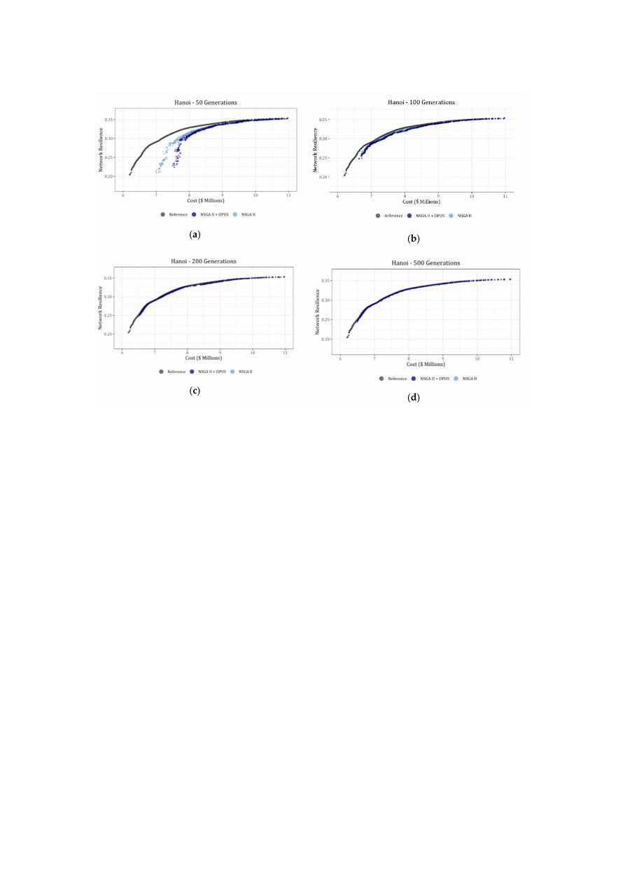
For the Hanoi network, the evolution of the PFs is shown in Figure
2
a–d, showing the results for
50, 100, 200, and 500 generations. In this first case, the NSGA-II algorithm showed a faster approach to
the benchmark front for the first 50 generations. However, when the algorithms reached approximately
100 generations, the di
fference among the approaches tends to reduce significantly. Additionally,
the greater di
fferences between the PFs occur during the first generations, but as soon as it overpasses
the 200 generations, they do not change considerably. This statement will be discussed later, aided by
the performance metrics.
Water 2020, 12, 3101
12 of 23
Figure 2.
Evolution of the PFs for the non-dominated sorting-based multi-objective evolutionary
algorithm (NSGA-II) algorithm (light blue) and the retrofitted NSGA-II with optimal power use
surface (OPUS) (dark blue) in comparison to the best-known PF (black) for Hanoi. (a) 50 generations;
(b) 100 generations; (c) 200 generations and (d) 500 generations.
In this case, it is important to highlight that the results for the Hanoi network could be a
ffected
by the number of available commercial diameters. Several authors have stated before that the
diameters’ list for this benchmark lacks for a higher diameter than the current one, which is 40 in [
11
].
Consequently, given that the OPUS design is made considering continuous diameters, it is not possible
to find a correspondingly good solution when the NSGA-II algorithm tries to round it to the nearest
diameter. Therefore, the e
ffect of the retrofitting process is not an advantage for the proposed algorithm,
and instead, it slows down its e
fficiency.
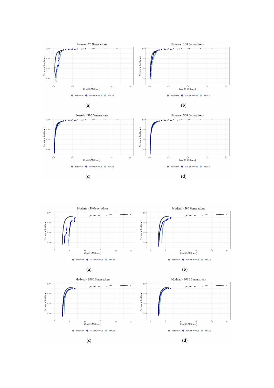
For the Fossolo network, the evolution of the PFs is shown in Figure
2
a–d, showing the results for
20, 100, 300, and 500 generations. In this case, the PF obtained using the proposed algorithm is closer
to the benchmark front than the obtained by using the NSGA-II by itself since the beginning of the
simulations. Additionally, there are some gaps presented in Figure
3
a, which are a consequence of the
penalty functions used to meet both velocity and pressure constraints. Despite the presence of these
gaps, as the algorithm evolves, they tend to disappear until the front is completed. Moreover, the most
significant changes in the fronts occurred in the first 200 to 300 generations, and after that, the PF did
not change significantly.
The evolution of the PFs for the Modena network is shown in Figure
4
a–d, showing the results
for 50, 500, 2000, and 4000 generations. Once again, the PF obtained using the proposed algorithm is
closer to the benchmark front than the obtained by using the NSGA-II by itself since the beginning of
the simulations. Analogous to the Fossolo network, Modena’s design is constrained by a maximum
velocity. Therefore, a penalty function was included in the algorithms, explaining the gaps observed in
the first 50 generations. In the following graphs, the PF is filled and do not show a significant variation
in the last generations.
Water 2020, 12, 3101
13 of 23
Figure 3.
Evolution of the PFs for the NSGA-II algorithm (light blue) and the retrofitted NSGA-II
with OPUS (dark blue) in comparison to the best-known PF (black) for Fossolo. (a) 20 generations;
(b) 100 generations; (c) 300 generations and (d) 500 generations.
Figure 4.
Evolution of the PFs for the NSGA-II algorithm (light blue) and the retrofitted NSGA-II with
Water 2020, 12, 3101
14 of 23
OPUS (dark blue) in comparison to the best-known PF (black) for Modena. (a) 50 generations;
(b) 500 generations; (c) 2000 generations and (d) 4000 generations.
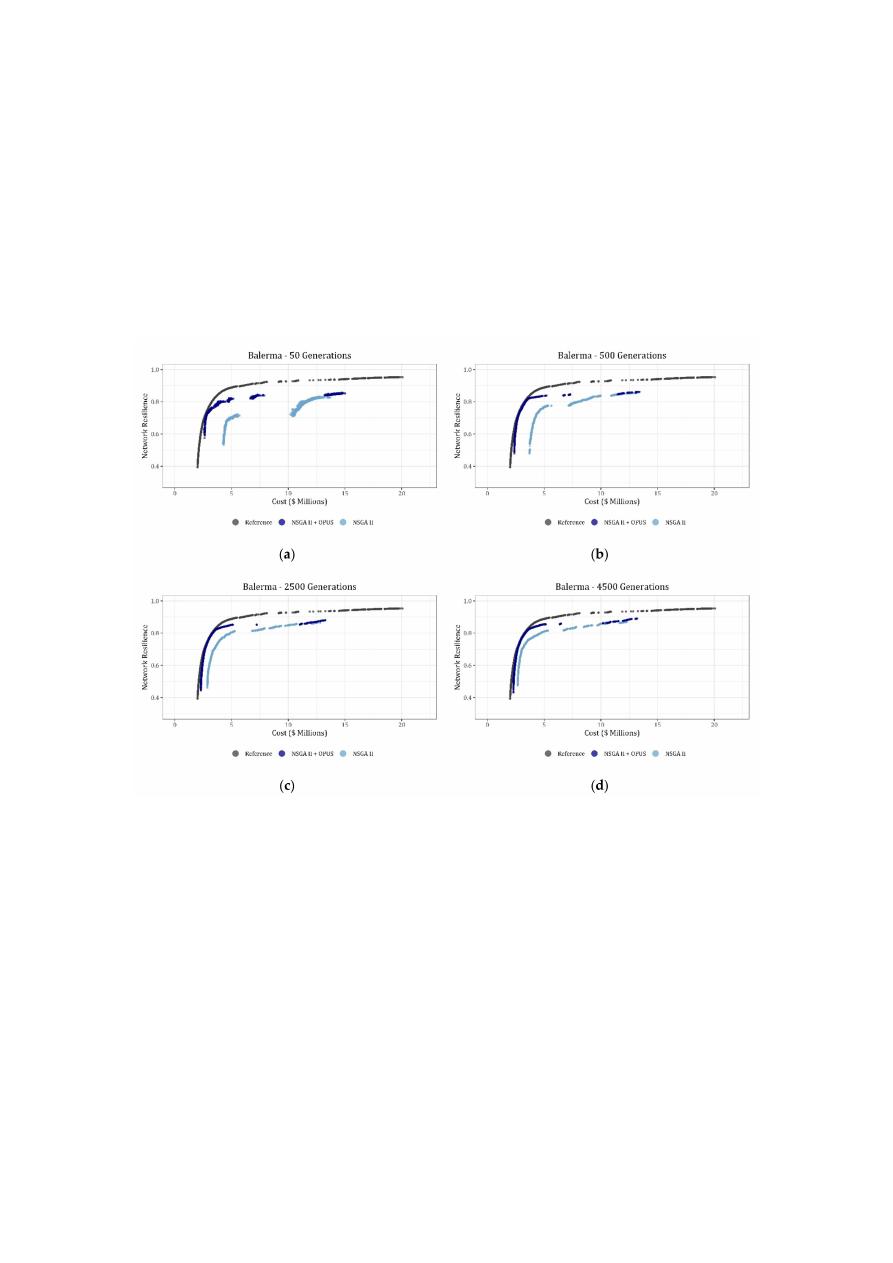
Finally, the evolution of the PFs for the Balerma network is shown in Figure
5
a–d, showing the
results for 50, 500, 2500, and 4500 generations. For this network, the proposed algorithm developed
with a significant advantage regarding the NSGA-II by itself, as it is shown in Figure
5
. Additionally,
the approximation of the algorithms described in this research could be closer to the best-known PF
if a higher number of generations is used. However, it is important to highlight the increase in the
e
fficiency of the NSGA-II when it is retrofitted by the OPUS algorithm aiming to reach a good solution
for the design of the network.
Figure 5.
Evolution of the PFs for the NSGA-II algorithm (light blue) and the retrofitted NSGA-II
with OPUS (dark blue) in comparison to the best-known PF (black) for Balerma. (a) 50 generations;
(b) 500 generations; (c) 2500 generations and (d) 4500 generations.
The size of the networks tested seems to have a direct impact on the increase of the e
fficiency
reached by the algorithm when it is retrofitted by an energy-based method such as OPUS. When a
medium network such as Hanoi was tested, the di
fference in the PF between the proposed algorithm
and the NSGA-II by itself was not as significant as they were when Balerma, a large water supply
system, was tested.
6.2. Results for Performance Metrics
The assessment of the performance of the tested algorithms was performed using hypervolume
(HV) and modified inverted generational distance (IGD
+). Thus, the evolution of the metrics for
NSGA-II and the proposed algorithm are shown in Figure
6
a–d, and Figure
7
a–d for the HV and IGD
+,
respectively, organized from the smallest (Hanoi) to the largest (Balerma) tested networks. In the
mentioned graphs, the results for NSGA-II are shown in red, the proposed algorithm in green, and the
corresponding value to the best-known PF is shown as a continuous red line.
Water 2020, 12, 3101
15 of 23
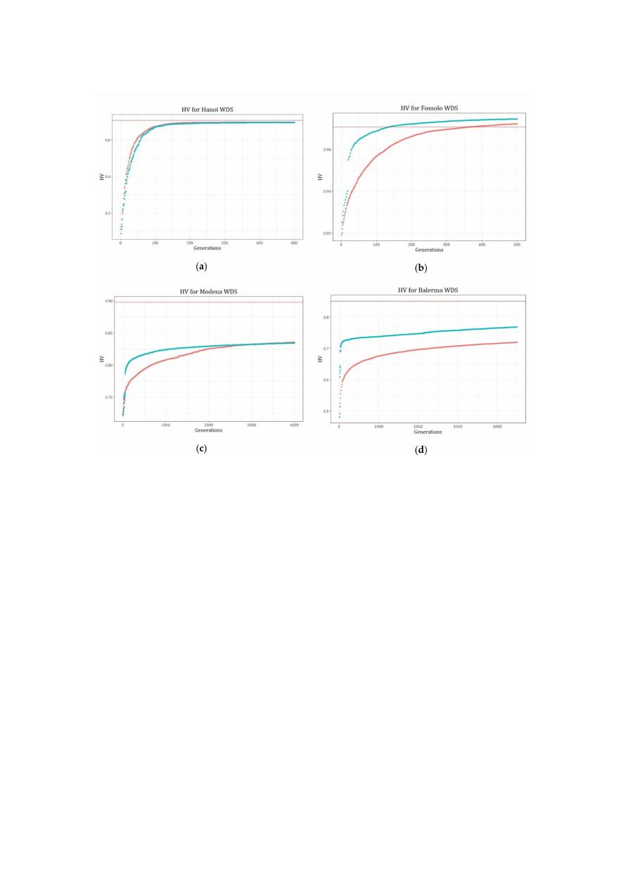
Figure 6.
Evolution of the hypervolume (HV) for assessing the results of the NSGA-II algorithm (red)
and the retrofitted NSGA-II with OPUS (green) in comparison to the hypervolume (HV) best-known
PF (continuous red line) for tested networks. (a) Hanoi; (b) Fossolo; (c) Modena and (d) Balerma.
Additionally, when HV is analyzed, the di
fferences between the best-known PF and the obtained
results were 1.83%, −0.35%, 7.10%, and 9.79% for Hanoi, Fossolo, Modena, and Balerma, respectively.
In this case, the resulting di
fferences are less than 10%, validating the quality of the results.
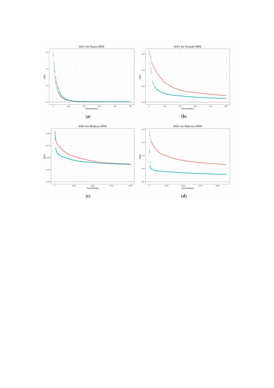
In the case of the IGD
+, given that the best-known PF corresponds to 0, it is expected that
high-quality designs are close to this value. Hence, the IGD
+ values obtained for the four tested cases
were 0.0041, 0.0045, 0.035, and 0.028, respectively, supporting the conclusion led by the HV.
Nevertheless, regarding the performance of the algorithms, the results for both HV and IGD
+
metrics show the advantage of the retrofitted algorithm respect to the NSGA-II itself, specifically during
the first generations, where the more significant gaps occur as a measurement of the acceleration in the
convergence rate of the algorithms. Moreover, the metrics show that for Hanoi and Modena networks,
both algorithms tend to converge to a similar value after a certain number of generations. However,
in Modena, the jump resulting from the feedback helps the proposed algorithm to stabilize in earlier
generations than NSGA-II by itself. Regarding Fossolo and Balerma, a similar result is observed, giving
a clear advantage to the proposed algorithm.
Water 2020, 12, 3101
16 of 23
Figure 7.
Evolution of the IGD
+ for assessing the results of the NSGA-II Algorithm (red) and the
retrofitted NSGA-II with OPUS (green) in comparison to the inverted generational distance (IGD
+)
best-known PF (continuous red line) for tested networks. (a) Hanoi; (b) Fossolo; (c) Modena and
(d) Balerma.
The quantification of the advantage of the proposed algorithm respect NSGA-II was performed
by determining the percentage di
fference between both. The latter was calculated in terms of the HV
showed in Figure
6
, resulting in a positive value the generations in which the retrofitted algorithm
obtained a higher HV than the evolutionary algorithm by itself, and a negative value otherwise. Hence,
the results for this approach is shown in Figure
8
a–d for the four tested networks.
In these plots, Hanoi was retrofitted with a frequency of 5 generations, which is reflected in the
oscillatory trend during the first 100 generations. Although the results for Hanoi showed this behavior,
the other case studies presented an evident trend in their results. Fossolo, Modena, and Balerma
showed a percentage di
fference of 2.07%, 3.32%, and 14.90% respectively in the generation number 20,
50, and 10 correspondingly. Moreover, the generation in which the maximum gap for the HV occurred
matches the time for the first feedback using the OPUS algorithm.
However, the gap between the tested algorithms tends to reduce in further feedbacks, until there
is a moment when there is not a significant di
fference in the HV from both algorithms as the number of
generations increases. Summarizing, this means that the proposed methodology has a major impact
the first time that feedback occurs, and later this e
ffect will tend to be reduced, making OPUS a good
hot-start for evolutionary algorithms.
Additionally, in Figure
8
, it is confirmed that the magnitude of the gaps obtained by using the
proposed algorithm increases with the size of the network, being 2.07% and 3.32% for Fossolo and
Modena networks correspondingly (intermediate to large WDN), and of 14.90% for Balerma network,
which is the largest of the tested systems.

Water 2020, 12, 3101
17 of 23
Figure 8.
Percentage di
fference for the HV between the results for NSGA-II and the proposed algorithm.
(a) Hanoi; (b) Fossolo; (c) Modena and (d) Balerma.
Furthermore, although several authors have proposed di
fferent approaches to the multi-objective
design problem for WDS, the results may vary in terms of e
fficiency, spread, and even the quality
of the solutions. Therefore, it is possible to reach slightly better solutions than the best-known PF
obtained by Wang et al. [
21
], except for those networks where their search space is small enough to
have a complete enumeration of the solutions, leading to a true PF [
22
].
As an exemplification, Bi et al. [
27
] presented a solution for Fossolo and Hanoi networks where
the hypervolume (HV) was greater than 0.95, which corresponded to the best-known PF established
by Wang et al. [
21
]. These solutions were accomplished using the multi-objective prescreened
heuristic sampling method (MOPHSM). A similar result was obtained by Yazdi et al. [
24
], where the
non-dominated sorting harmony search di
fferential evolution (NSHSDE) algorithm was implemented,
reaching for Fossolo network a PF that was better than the best-known PF in terms of the resilience of
the solutions. In a most recent approach, Cunha and Marques [
22
] established new best-known PF
for nine benchmark networks, classified as medium to large sizes using the multi-objective simulated
annealing (MOSA) algorithm, including the Fossolo network. Finally, in this research, authors also
reached slightly better solutions for the Fossolo network in terms of its resilience, using the proposed
retrofitted NSGA-II algorithm with OPUS as well as the NSGA-II itself. This is validated in Figure
5
b,
where the HV for both approaches are compared with the best-known results.
6.3. Statistical Analysis of the Results
Due to the inherent randomness of the NSGA II algorithm, it was necessary to perform a statistical
analysis of the behavior of the PFs. In such a manner, the e
ffect of using OPUS could be distinguished
Water 2020, 12, 3101
18 of 23
from mere chance. This evaluation considered the two smaller networks, Hanoi and Fossolo, to assess
the performance of the fronts due to their computational speed.
The examination consisted of the execution of 30 simulations of each algorithm for both WDS so
that the results drawn from it were statistically valid. Therefore, the values for the metrics as functions
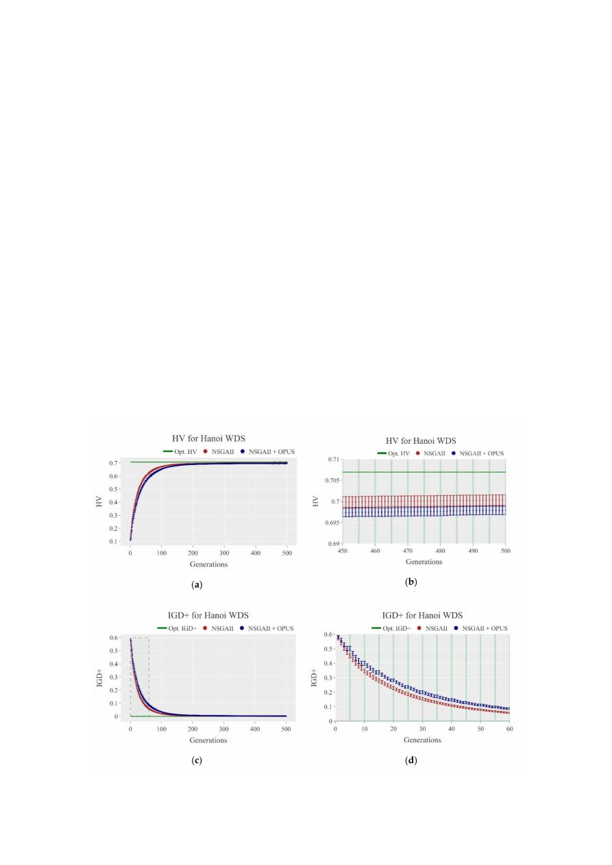
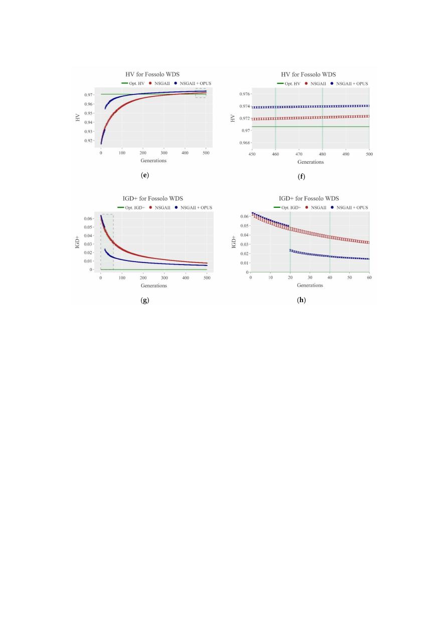
of the generations are shown in Figure
9
a–h. Each point has a 95% confidence interval calculated using
the data from the simulations and a Student’s t distribution with 29 degrees of freedom.
The confidence intervals provide further insights into the development of the PFs. First, the width
of the intervals decreased as the algorithm developed. The intervals were wider at the beginning of
the process because the solutions were random. Hence, as they were far from optimal, the variance
tended to increase. Whereas, at later stages, it was harder to find better solutions as the PFs stabilized.
Secondly, the widths of the intervals were small compared to the values of the metrics, which indicated
low uncertainty on the results. Although the solutions sampled by NSGA-II were random, the overall
behavior of the PFs was stable. Therefore, it produced very similar HV and IGD
+ results for different
simulations, which, consequently, generated low standard deviations and narrow confidence intervals.
Finally, for any generation, after the first OPUS retrofitting occurred, the confidence intervals of
both methodologies did not overlap, which indicated that the average values of the metrics were
statistically di
fferent.
Even though a rigorous statistical analysis requires multiple simulations, the overall behavior
of the smaller networks’ PFs (represented by the metrics and their variance) indicates that a single
simulation of both algorithms is highly representative of their performance. Therefore, for Modena and
Balerma, we implemented this one-simulation approach. These bigger networks involve extensive time
and computational cost, and, as previously stated, one simulation is enough to compare su
fficiently
the algorithms’ functioning.
Figure 9. Cont
.
Water 2020, 12, 3101
19 of 23
Figure 9.
The 95% confidence intervals for performance metrics at each generation for multiple
executions of the NSGA-II and the OPUS retrofitted algorithms. (a) HV for Hanoi; (b) stabilized HV
for Hanoi; (c) IGD
+ for Hanoi; (d) IGD+ for Hanoi during the first generations; (e) HV for Fossolo;
(f) stabilized HV for Fossolo; (g) IGD
+ for Fossolo; and (h) IGD+ for Fossolo during the first generations.
The graphs at the right are the zoom of the dashed boxes of the graphs on the left. The green vertical
lines indicate the generations in which OPUS was used.
7. Conclusions
The multi-objective optimal design of WDN, considering the capital costs and the reliability of
the systems, was addressed by comparing two approaches: a traditional NSGA-II algorithm and a
proposed algorithm in which this evolutionary algorithm was retrofitted with an energy-based method.
These methodologies were tested into four well-known design benchmarks (Hanoi, Fossolo, Modena,
and Balerma), and then compared their performance and quality of solutions to the corresponding
best-known PF [
21
] using two metrics: hypervolume (HV) and modified inverted generational distance
(IGD
+). These metrics were selected because they are unary metrics with uniformity, convergence, and
spread quality properties [
38
].
Before the two algorithms were tested in the case studies, a calibration procedure was performed.
Although neither an exhaustive nor an optimal search of the values of the parameters were accomplished
given the scope of the paper, the set of determined values sought to make a better approximation to the
best-known Pareto front within the recommended ranges for each parameter. Hence, after performing
several simulations testing di
fferent values for each parameter within their corresponding range for
each tested network, the values were selected after a visual inspection of the resulting PFs pursuing
three characteristics: the spread, distribution, and convergence to the optimal PF. For further research,
a wider range of parameters could be tested to analyze their performance in the development of the
NSGA-II algorithm.
The set of calibrated parameters were used for both NSGA-II and the retrofitted algorithm to make
a plausible comparison between them. Moreover, the retrofitting frequency, or parameter m, was tuned

Water 2020, 12, 3101
20 of 23
for each network seeking to increase the performance of the proposed algorithm. For further research,
it is recommended to test the overall e
ffect of this parameter over the other NSGA-II parameters, as
well as its correlation with the size of the networks. Additionally, the calibration procedure could be
improved by implementing a systemic approach if the scope of the study is to achieve better PF rather
than improving the e
fficiency of the algorithm.
Regarding Hanoi, the NSGA-II algorithm showed better results than the retrofitted algorithm.
This occurs given that the maximum diameter available for this benchmark is not enough to reach a
near-optimal design when using energy-based methods, as it has been stated by several authors such
as Saldarriaga et al. [
11
]. Therefore, when OPUS is used to make feedback on NSGA-II, as it performs a
continuous design, the input diameters resulting from this process that are greater than 40 in. are going
to be rounded o
ff to that value. Hence, the proposed algorithm will lose efficiency because a loop-wide
behavior, in which the continuous design from OPUS will try to reach a near-optimal solution with a
higher diameter, and NSGA-II will try to round it to 40 in.
Despite the results obtained in Hanoi, in the remaining study cases, the proposed algorithm
reached closer solutions to the best-known PF in a more e
fficient manner than a traditional NSGA-II.
Moreover, the feedback process of the proposed algorithm tended to accelerate the convergence of
the evolutionary algorithm, which is reflected in the gaps in the HV obtained in the first retrofitting
generation for each network: 2.07% in Fossolo, 3.32% in Modena, and 14.90% in Balerma. However,
these impacts were substantial only the first time the algorithm was retrofitted, and in further feedbacks,
the magnitude of the gaps started to reduce until there is no significant di
fference between the HV
evolution for the tested algorithms.
The previous analysis also made evident an important conclusion: when the PFs were compared,
the size of the network seems to play a key role in the e
fficiency of the proposed algorithm. Hence,
when the network is bigger, the impact of the feedback is more significant in the improvement of the
solutions. Therefore, the e
ffect of using OPUS for retrofitting the NSGA-II was higher when Balerma
was analyzed (14.90% in the first feedback) rather than Fossolo, which was an intermediate-size
network (2.07% in the first feedback).
Regarding the HV and IGD
+, which were the metrics used for assessing the performance and
quality of the algorithms, it can be concluded that they were useful to quantify the closeness of the
results obtained against the best-known PF for each network. For HV, the di
fferences between the value
obtained for the best-known PF and the results were 1.83%, −0.35%, 7.10%, and 9.79% correspondingly
for Hanoi, Fossolo, Modena, and Balerma. In the case of the IGD
+, considering that the best-known
PF corresponds to 0, then the values obtained for the four tested cases were 0.0041, 0.0045, 0.035, and
0.028 correspondingly. Hence, it can be concluded that the proposed algorithm can reach PFs with a
di
fference of less than 10% regarding the benchmark fronts.
In the results for Fossolo, the HV at the last generation for the proposed algorithm had a di
fference
of −0.35% regarding the best-known PF established by Wang et al. [
21
], representing a slightly better
solution. Similar situations have been exposed by Bi et al. [
27
], Yazdi et al. [
24
], and Cunha and
Marques [
22
]. Even though it is possible to improve the quality of the solution slightly in medium,
intermediate, and large-size networks, there are small networks in which is possible to perform a
complete enumeration given the size of their search space, leading to a true PF and consequently
avoiding further improvements [
22
]. For further research, it is recommended to test a higher number
of networks while considering more sizes and topologies than the ones considered in this paper,
to explore a potential relationship between the size and characteristics of the networks. Hence, the
user of the algorithms will be capable of establishing the potential benefit of using an energy-based
method to retrofit an evolutionary algorithm, in this case, NSGA-II, before its implementation.
Additionally, the evolution of the metrics along with the number of generations made evident the
behavior of the tested algorithms. During the first generations, the most significant changes in the
metrics occurred; as the methodologies developed, the change in the metrics got less significant until
they stabilized, meaning that a set of solutions (PF) was reached. This behavior can be oriented to take

Water 2020, 12, 3101
21 of 23
advantage of two aspects: (1) the use of an approach that allows navigating faster into the search space,
as in this case, an energy-based input; and (2) the determination of an optimal number of generations
required to reach a near-optimal solution, avoiding additional computational e
fforts.
The statistical analysis of the PFs’ metrics indicated that the overall behavior of the PFs for
di
fferent simulations was stable. Consequently, the variances of the metrics for every generation
of the algorithms was small, and it decreased as the fronts converged in later generations. Thus,
the confidence intervals calculated with these variances were su
fficiently narrow to discard multiple
simulations. Conversely, it was possible to use a one-simulation approach for every method and still be
able to compare them validly. Furthermore, the confidence intervals did not overlap, which indicates
that the average values of the metrics were statistically di
fferent.
The approach of energy-based methods such as OPUS, to WDS optimal design problem, has the
capabilities of reaching near-optimal solutions in a reduced number of iterations; besides, it represents a
practical approach for engineers who are not familiarized with optimization procedures. Furthermore,
in the algorithm presented in this paper, the capabilities of OPUS are extended to a wider range,
allowing it to be a high-quality and feasible start for an evolutionary procedure. Thus, the convergence
rate of these algorithms can be speeded up, achieving closer solutions to benchmark PFs, especially in
larger networks.
Finally, the proposed algorithm proved that it is feasible to reach a near-optimal set of solutions
(or PF) close enough to the benchmark front in an e
fficient manner. Given that the most considerable
e
ffect of the feedback is obtained during the first time the algorithm is retrofitted, derived methodologies
should focus on using energy-based methods to perform a hot-start for evolutionary algorithms.
Afterward, in further stages of the algorithm, the feedback procedure can be modified to maintain a
significant e
ffect on its convergence. However, the proposed methodology presented in this research
ensures a good approach to the optimal design problem considering di
fferent objectives related to the
cost and the reliability of the network.
Supplementary Materials:
The following are available online at
https:
//zenodo.org/record/4198907#
.X6KOUIhKhPY
. Approximations to the Best-known PFs using NSGA-II retrofitted by OPUS for Hanoi, Fossolo,
Modena, and Balerma, Approximations to the Best-known PFs using NSGA-II for Hanoi, Fossolo, Modena and
Balerma, HV and IGD
+ for Hanoi, Fossolo, Modena and Balerma.
Author Contributions:
J.S. and D.P. conceived the algorithm and both guided and supervised the research process;
D.P., C.S., A.G., M.A.G., and J.S. wrote the paper; M.A.G. performed the literature review; D.P. implemented the
algorithm using MATLAB software; C.S. and A.G. performed the simulations, analyzed the results and performed
the statistical analysis; A.G. developed tools for calculating the used metrics and analyzed the results. All authors
have read and agreed to the published version of the manuscript.
Funding:
This research received no external funding.
Acknowledgments:
The authors acknowledge Yves Filion for the support and guidance of Diego Páez’s research.
Additionally, the authors acknowledge the following undergraduate students who participated in the early stages
of the research: Carlos Martinez, Andrés Avila, Lina Cárdenas, Silvana Téllez, Luisa Bonilla, and Federico Cruz.
Conflicts of Interest:
The authors declare no conflict of interest.
References
1.
Yates, D.; Templeman, A.; Bo
ffey, T. The computational complexity of the problem of determining least
capital cost designs for water supply networks. Eng. Optim. 1984, 7, 143–155. [
CrossRef
]
2.
Artina, S. Use of mathematical programming techniques in designing hydraulic networks. Meccanica 1973, 8,
158–167. [
CrossRef
]
3.
Reca, J.; Martínez, J.; López, R. A Hybrid Water Distribution Networks Design Optimization Method Based
on a Search Space Reduction Approach and a Genetic Algorithm. Water 2017, 9, 845. [
CrossRef
]
4.
Cunha, M.; Sousa, J. Water Distribution Network Design Optimizaction: Simulated Annealing Approach.
J. Water Resour. Plan. Manag. 1999, 125, 215–221. [
CrossRef
]
5.
Geem, Z.W. Multiobjective optimization of water distribution networks using fuzzy theory and harmony
search. Water 2015, 7, 3613–3625. [
CrossRef
]

Water 2020, 12, 3101
22 of 23
6.
Eusu
ff, M.M.; Lansey, K.E. Water distribution network design using the shuffled frog leaping algorithm.
In Proceedings of the World Water and Environmental Resources Congress, Orlando, FL, USA, 20–24 May
2001; pp. 210–225. [
CrossRef
]
7.
Geem, Z.W. Particle-swarm harmony search for water network design. Eng. Optim. 2009, 41, 297–311.
[
CrossRef
]
8.
Wu, I. Design of drip irrigation main lines. J. Irrig. Drain. Eng. 1975, 101, 265–278.
9.
Featherstone, R.E.; El-Jumaily, K.K. Optimal diameter selection for pipe networks. J. Hydraul. Eng. 1983, 109,
221–234. [
CrossRef
]
10.
Takahashi, S.; Saldarriaga, J.; Hernández, F.; Díaz, D.; Ochoa, S. An energy methodology for the design
of water distribution systems. In Proceedings of the Proceedings of the World Environmental and Water
Resources Congress, Providence, RI, USA, 16–20 May 2010.
11.
Saldarriaga, J.; Páez, D.; Salcedo, C.; Cuero, P.; López, L.L.; León, N.; Celeita, D. A Direct Approach for the
Near-Optimal Design of Water Distribution Networks Based on Power Use. Water 2020, 12, 1037. [
CrossRef
]
12.
Deb, K.; Pratap, A.; Agarwal, S.; Meyarivan, T. A fast and elitist multiobjective genetic algorithm: NSGA-II.
IEEE Trans. Evol. Comput. 2002, 6, 182–197. [
CrossRef
]
13.
Farmani, R.; Savic, D.A.; Walters, G.A. “EXNET” Benchmark Problem for Multi-Objective Optimization of
Large Water Systems. In Proceedings of the Modelling and Control for Participatory Planning and Managing
Water Systems, IFAC Workshop, Venice, Italy, 29 September–1 October 2004.
14.
Prasad, T.; Park, N. Multiobjective Genetic Algorithms for Design of Water Distribution Networks. J. Water
Resour. Plan. Manag. 2004, 130, 73–82. [
CrossRef
]
15.
Atkinson, S.; Farmani, R.; Memon, F.A.; Butler, D. Reliability indicators for water distribution system design:
Comparison. J. Water Resour. Plan. Manag. 2014, 140, 160–168. [
CrossRef
]
16.
Monsef, H.; Naghashzadegan, M.; Farmani, R.; Jamali, A. Deficiency of Reliability Indicators in Water
Distribution Networks. J. Water Resour. Plan. Manag. 2019, 145, 1–10. [
CrossRef
]
17.
Raad, D.N.; Sinske, A.N.; van Vuuren, J.H. Comparison of four reliability surrogate measures for water
distribution systems design. Water Resour. Res. 2010, 46, 1–11. [
CrossRef
]
18.
Creaco, E.; Fortunato, A.; Franchini, M.; Mazzola, M.R. Comparison between entropy and resilience as
indirect measures of reliability in the framework of water distribution network design. Procedia Eng. 2014,
70, 379–388. [
CrossRef
]
19.
Zhan, X.; Meng, F.; Liu, S.; Fu, G. Comparing performance indicators for assessing and building resilient
water distribution systems. J. Water Resour. Plan. Manag. 2020, 146, 1–8. [
CrossRef
]
20.
Raad, D.; Sinske, A.; Van Vuuren, J. Robust multi-objective optimization for water distribution system design
using a meta-metaheuristic. Int. Trans. Oper. Res. 2009, 16, 595–626. [
CrossRef
]
21.
Wang, Q.; Guidolin, M.; Savié, D.; Kapelan, Z. Two-Objective Design of Benchmark Problems of Water
Distribution System via MOEAs: Towards the Best-Known Approximation to the True Pareto Front. J. Water
Resour. Plan. Manag. 2015, 141, 04014060. [
CrossRef
]
22.
Cunha, M.; Marques, J. A New Multiobjective Simulated Annealing Algorithm—MOSA-GR: Application to
the Optimal Design of Water Distribution Networks. Water Resour. Res. 2020, 56, e2019WR025852. [
CrossRef
]
23.
Creaco, E.; Franchini, M. Low level hybrid procedure for the multi-objective design of water distribution
networks. Procedia Eng. 2014, 70, 369–378. [
CrossRef
]
24.
Yazdi, J.; Choi, Y.H.; Kim, J.H. Non-dominated sorting harmony search di
fferential evolution (NS-HS-DE): A
hybrid algorithm for multi-objective design of water distribution networks. Water 2017, 9, 587. [
CrossRef
]
25.
Keedwell, E.; Khu, S.T. Novel cellular automata approach to optimal water distribution network design. J.
Comput. Civ. Eng. 2006, 20, 49–56. [
CrossRef
]
26.
Kang, D.; Lansey, K. Revisiting Optimal Water-Distribution System Design: Issues and a Heuristic Hierarchical
Approach. J. Water Resour. Plan. Manag. 2012, 138, 208–217. [
CrossRef
]
27.
Bi, W.; Dandy, G.C.; Maier, H.R. Use of domain knowledge to increase the convergence rate of evolutionary
algorithms for optimizing the cost and resilience of water distribution systems. J. Water Resour. Plan. Manag.
2016
, 142, 1–12. [
CrossRef
]
28.
Liu, H.; Shoemaker, C.A.; Jiang, Y.; Fu, G.; Zhang, C. Preconditioning Water Distribution Network
Optimization with Head Loss–Based Design Method. J. Water Resour. Plan. Manag. 2020, 146, 04020093.
[
CrossRef
]

Water 2020, 12, 3101
23 of 23
29.
Bi, W.; Dandy, G.C.; Maier, H.R. Improved genetic algorithm optimization of water distribution system
design by incorporating domain knowledge. Environ. Model. Softw. 2015, 69, 370–381. [
CrossRef
]
30.
Todini, E. Looped water distribution networks design using a resilience index based heuristic approach.
Urban Water 2000, 2, 115–122. [
CrossRef
]
31.
Ochoa, S. Diseño Optimizado de Redes de Distribución de Agua Potable con Base en el Concepto Energético
de Superficie Óptima de Gradiente Hidráulico (Optimal Water Distribution Network Design Based on the
Optimal Hydraulic Gradient Surface Energetic Concept). Master’s Thesis, Universidad de los Andes, Bogota,
Columbia, 2009.
32.
Saldarriaga, J.; Páez, D.; León, N.; López, L.L.; Cuero, P. Power use methods for optimal design of WDS:
History and their use as post-optimization warm starts. J. Hydroinformatics 2015, 17, 404–421. [
CrossRef
]
33.
Wang, Q.; Wang, L.; Huang, W.; Wang, Z.; Liu, S.; Savi´c, D.A. Parameterization of NSGA-II for the optimal
design of water distribution systems. Water 2019, 11, 971. [
CrossRef
]
34.
Deb, K.; Agrawal, R.B. Simulated Binary Crossover for Continuous Search Space. Complex Syst. 1994, 9,
115–118.
35.
Deb, K.; Deb, A. Analysing mutation schemes for real-parameter genetic algorithms. Int. J. Artif. Intell.
Soft Comput. 2014, 9, 115–148. [
CrossRef
]
36.
Rossman, L.A. Epanet 2. User’s Manual; Water Supply and Water Resources Division National Risk
Management Research Laboratory: Cincinnati, OH, USA, 2000.
37.
Paez, D.; Salcedo, C.; Avila, A.; Filion, Y.; Saldarriaga, J. Improving Convergence Rate of NSGA II with
Intermittent Feedback from Energy Based Methods for Design of Water Distribution Systems. In Proceedings
of the 1st International WDSA
/CCWI Joint Conference, Kingston, ON, Canada, 23–25 July 2018.
38.
Li, M.; Yang, S.; Liu, X. Diversity comparison of Pareto front approximations in many-objective optimization.
IEEE Trans. Cybern. 2014, 44, 2568–2584. [
CrossRef
]
39.
Zitzler, E.; Thiele, L. Multiobjective evolutionary algorithms: A comparative case study and the strength
Pareto approach. IEEE Trans. Evol. Comput. 1999, 3, 257–271. [
CrossRef
]
40.
Ishibuchi, H.; Masuda, H.; Tanigaki, Y.; Nojima, Y. Modified distance calculation in generational distance
and inverted generational distance. In Proceedings of the International Conference on Evolutionary
Multi-Criterion Optimization, Guimarães, Portugal, 29 March–1 April 2015.
41.
Fujiwara, O.; Khang, D.B. A two-phase decomposition method for optimal design of looped water distribution
networks. Water Resour. Res. 1990, 26, 539–549. [
CrossRef
]
42.
Bragalli, C.; D’Ambrosio, C.; Lee, J.; Lodi, A.; Toth, P. On the optimal design of water distribution networks:
A practical MINLP approach. Optim. Eng. 2012, 13, 219–246. [
CrossRef
]
43.
Reca, J.; Martínez, J. Genetic algorithms for the design of looped irrigation water distribution networks.
Water Resour. Res. 2006, 42, W05416. [
CrossRef
]
Publisher’s Note:
MDPI stays neutral with regard to jurisdictional claims in published maps and institutional
a
ffiliations.
© 2020 by the authors. Licensee MDPI, Basel, Switzerland. This article is an open access
article distributed under the terms and conditions of the Creative Commons Attribution
(CC BY) license (http:
//creativecommons.org/licenses/by/4.0/).
