Urban Drainage Network Rehabilitation Considering Storm Tank Installation and Pipe Substitution.

water

Article

Urban Drainage Network Rehabilitation Considering
Storm Tank Installation and Pipe Substitution

Ulrich A. Ngamalieu-Nengoue

1

, Pedro L. Iglesias-Rey

1,

* , F. Javier Martínez-Solano

1

,

Daniel Mora-Meliá

2

and Juan G. Saldarriaga Valderrama

3

1

Department of Hydraulic Engineering and Environment, Universitat Politècnica de València. Camino de

Vera s/n, 46022 Valencia, Spain; ngamaleuulrich@yahoo.fr (U.A.N.-N.); jmsolano@upv.es (F.J.M.-S.)

2

Department of Engineering and Construction Management, Facultad de Ingeniería, Universidad de Talca,
3340000 Talca, Chile; damora@utalca.cl

3

Department of Hydraulic Engineering and Environment, Water Supply and Sewerage System Research
Center (CIACUA), University of Los Andes, Cra 1 # 18A-11, Bogota D.C., Colombia;
jsaldarr@uniandes.edu.co

*

Correspondence: piglesia@upv.es; Tel.: +34-96-387-70-00 (ext. 86111)

Received: 21 January 2019; Accepted: 6 March 2019; Published: 12 March 2019

Abstract:

The drainage networks of our cities are currently experiencing a growing increase in runoff

flows, caused mainly by the waterproofing of the soil and the effects of climate change. Consequently,
networks originally designed correctly must endure floods with frequencies much higher than those
considered in the design phase. The solution of such a problem is to improve the network. There are
several ways to rehabilitate a network: conduit substitution as a former method or current methods
such as storm tank installation or combined use of conduit substitution and storm tank installation.

To find an optimal solution, deterministic or heuristic optimization methods are used. In this paper,

a methodology for the rehabilitation of these drainage networks based on the combined use of the
installation of storm tanks and the substitution of some conduits of the system is presented. For this,
a cost-optimization method and a pseudo-genetic heuristic algorithm, whose efficiency has been

validated in other fields, are applied. The Storm Water Management Model (SWMM) model for

hydraulic analysis of drainage and sanitation networks is used. The methodology has been applied
to a sector of the drainage network of the city of Bogota in Colombia, showing how the combined use
of storm tanks and conduits leads to lower cost rehabilitation solutions.

Keywords:

drainage network; climate change; rehabilitation; optimization; SWMM

1. Introduction

One of the main problems related to urban drainage systems are the frequent flooding events

in urban areas. Various factors can cause these events, such as pipe size, structural failures in
the system, objects causing obstructions or an increase in rainfall intensity due to climate change
inducing increased runoff flow. Climate change undoubtedly affects the intensity and frequency of
meteorological phenomena of present days, including a gradual increase in rainfall intensities in many
cities throughout the world, making systems initially well designed begin to fail.

In order to have a better control over the systems and prevent the occurrence of urban flooding

events, many mechanisms have been implemented to reduce runoff and increase the capacity of the
system. Certainly, one of the most used methods in the last years has been the implementation of storm

water detention tanks (STs). These methods refer to the installation of devices in the urban area that

can hold back the flow that cannot be evacuated by the system. Later, when the system has regained
its transport capacity, the devices return the water to the sewerage system for correct evacuation.

Water 2019, 11, 515; doi:10.3390/w11030515

www.mdpi.com/journal/water

Water 2019, 11, 515

2 of 22

Howard [

1

] published one of the first works related to STs where it is established that the

effectiveness of the STs combined with Wastewater Treatment Plants (WTP) to control runoff depends
on STs and WTP’s capacity as well as the duration and volume of the precipitation events they must
control. Howard’s paper also lays out the possibility of using computational tools for the analysis of
these devices. His work focused on the usage of probabilistic methods based on precipitation data.

These water storage structures are built to retain a portion of the just-fallen rainwater, a portion

that varies according to every storm. Di Toro and Small [

2

] posited a statistical method based on a

probabilistic characterization of both rainwater and runoff that predicts the behavior of the storm water

control devices. The long-term behavior of a ST is determined based on its size, operation method
and both runoff and precipitation statistical characteristics. Based on these, Di Toro and Small studied
the filling, storage and emptying of the retaining structures; flow variations caused by storm water;
and first flush’s implications regarding water quality.

Early ST sizing methods were based on roughly simplified methods since simulation techniques

require a high computational effort in terms of time and memory. Loganathan et al. [

3

] presented a

simplified method that could estimate ST’s capacity accounting for previous storms. This method is
based on exponential probability density functions for the main hydrological variables involved (runoff

volumes, runoff duration, time between events). These functions are used to generate a new statistical

distribution that can estimate WTP’s capacity and retention volume for a given risk level. One of the
main advantages of this method is that it permits us to determine the preliminary volume for an ST.

With the same focus, Meredith et al. [

4

] developed a procedure based on all available historical data for

the dimension of a runoff storage structure. The dimensioning process uses the water quality concept
because all runoff must pass through the cleaning water process in the WTP. The method was tested in
several industrial areas, but it is limited to small areas where rational methods can be applied.

Most of these studies were focused on the treatment of rainwater runoff before the water enters

the network. Due to urban area space restrictions, alternative systems for the treatment of runoff water
are needed. For this, Takamatsu et al. [

5

] presented the design of a rainwater storage system as part

of the complementary structure of road drainage. They developed a mathematical model based on
the hydraulic principals to estimate the efficiency of the pollutant elimination. The main idea was to
evaluate the efficiency of a rectangular runoff ST removing suspended solids. In order to validate the
mathematical model, a scaled (1/5) network model was built, on which several tests were run to study
the influence of different inflows, functioning frequency and pollutant concentrations. The temporal
concentration of suspended solids at the exit and the efficiency of the conceptual model were compared.

They concluded that there is a correlation between the detention time and the removal efficiency.

Similar studies to Takamatsu et al. have been done to study the behavior of several draining areas

under different rainfall scenarios. De Martino et al. [

6

] proposed the usage of STs as structures that

enable controlling the impact of the first-rain contamination, which has the highest pollutant load.

As the design of this system depends on a large number of parameters, they consider that the design is

not completely defined. In order to study the influence that the rainwater might have, De Martino et al.
made several simulations with different rainfall-time series in Campania (Italy). This study made an
analysis of the hydrographs and pollutographs generated for several network and tank configurations.

The results showed that the rainfall does not have a direct influence in the reduction of pollutant

concentration. Based on this, a new methodology for the preliminary design of STs was presented.

In line with analyzing different rainfall amounts, Li et al. [

7

] analyzed 16 different rain events in

three drainage areas. The objective of this study was to analyze the effect of a detention tank’s location
on the polluted load reduction, mainly particles and metals. Thus, Fu et al. [

8

] presented a model

for optimum distribution of the STs in order to minimize the effect of new residential zones on the
discharge water quality. The developed model considered three working scenarios; optimum flow
control, minimization of deposit’s distribution and a combination of both. A step beyond was made
by Vanrolleghem et al. [

9

], who proposed a real time control system to manage the quality of water

poured in the collectors in order to comply with the European Water Framework.

Water 2019, 11, 515

3 of 22

Most of the previous works about the usage of STs are focused on the issue of maximizing

the quality of poured water, not to control the potential overflows that may occur due to excessive
rainwater, but some studies have been carried out in order to show that STs can also reduce floods.
One of the first studies that relate the usage of STs with the rainwater variation due to climate change

was done by Andrés-Domenech et al. [

10

]. The study focused on the effects originating from changes in

the rainfall regimes on the efficiency of the actual drainage systems. The proposed analytical statistical
model permits us to evaluate the overflow reduction efficiency and the retention tank’s volumetric
efficiency as a function of the expected climate behavior and urban basins. The tank’s efficiency
sensitivity is evaluated under the analysis of certain changes in the precipitation. The results show the
ability of STs to partially mitigate the resulting effects of climate change. Andrés-Domenech et al. based
their work in the same approach as Butler and Schütze [

11

]: integrate simulation models to obtain an

optimum control of the sanitary draining systems. For this purpose, Butler and Schütze developed a
model (SYNOPSIS) consisting of a series of sub-models of the sewage network, the treatment plant and
the behavior of the natural stream over which the system’s evacuation will be made. These sub-models,
together with a developed control module, allow the development of water control strategies in order
to minimize the impact on the water evacuation. The use of simulation techniques is simple for
urban wastewaters. Moreover, the simulation techniques enable water control solutions that were not

possible by the classic simplified methods. This work was extended by Fu et al. [

8

] taking into account

the optimization of urban wastewaters as a multi-objective problem. For this, they used a powerful
multi-objective genetic model called NSGA II [

12

] that allows obtaining the Pareto’s front for several

optimum solutions. For the same topic, Wang et al. [

13

] proposed a two-stage optimization framework

to find an optimal scheme for STs using the storm water management model (SWMM) [

14

]. As a result,

the authors conclude that the use of STs not only reduces flooding, but also the total suspended solids.

Drainage network rehabilitation is a necessary operation to adapt an insufficient network to the

new climatologic and environmental conditions. There are several ways to rehabilitate a drainage
network with difficulties in the compliance of its design specifications. Traditional ones consist
of pipes replaced with larger pipes. A newly developed option is the introduction of STs in the
network to store water during the storm, draining it after the extreme events have passed. In this
regard, Gaudio et al. [

15

] proposed a methodology for the hydraulic rehabilitation of urban drainage

networks combining a hydraulic analysis model, a data base of rainfall events and a series of synthetic
hyetographs. The results statistically analyze the possible places where the flood occurs and the
influence that the roughness of the pipes can have on it.

Considering the rehabilitation using pipe replacement and other actions, Sebti et al. [

16

] proposed

an algorithm to analyze the benefits of combining pipe substitution with other solutions installed to
reduce the runoff. However, Sebti et al. did not consider hydraulic models to analyze the consequences
of rehabilitation works in the network. Instead, they used the simplex algorithm for the optimization.

Then, Ugarelli and Di Federico [

17

] calculated the economic balance between replacing damaged

infrastructures or maintaining them for a certain period of time.

The rehabilitation of drainage networks based on the mere substitution of pipes is an approach

that has been traditionally carried out. However, this solution is not very applicable in consolidated
cities in which the replacement of large parts of the network interferes with other services already
installed and generates social problems for the population such as noise, inconvenience or traffic jams.

That is why this work proposes a combined use of the installation of STs and the replacement of pipes.
This is intended not only to reduce investment costs, but also to minimize the impact that changes

may have on citizens.

In short, the objective of this paper is to propose a methodology for the rehabilitation of

drainage networks that combines the installation of STs with the replacement of pipes. To do
this, the mathematical model of the network is the starting point, using SWWM to conduct the
hydraulic analysis and a pseudo-genetic optimization algorithm (PGA) [

18

] to find the best solutions.

The connection between the hydraulic calculation model and the optimization algorithm will be carried

Water 2019, 11, 515

4 of 22

out through an adaptation of the SWMM calculation toolkit done by Martínez-Solano et al. [

19

] in

order to reduce the calculation time.

The solution of the optimization problem requires an elevated number of decision variables (DVs)

generating a large space of feasible and unfeasible solutions. This search space entails not only a big
computational effort, but also may cause the method to fall at local minima, limiting the ability to
find the best solution. A reduction in the size of the problem and, subsequently, in the size of the
search space might help the convergence of the method. In this paper, a methodology for the reduction
of number of DVs based on pre-selection of potential locations of STs and the selection of conduits

potentially substitutable is proposed. This is a worthwhile contribution because reducing the size of

the search space and improving searching mechanisms are listed as current research challenges in the
application of optimization algorithms to real world problems [

20

,

21

].

The methodology has been validated in several networks. Although this paper presents the

results of application to the E-Chicó sector of the drainage network of Bogotá (Colombia), some model
files and additional case studies can be found in the supplementary material.

2. Problem Formulation

In order to formulate the problem of optimizing the rehabilitation of drainage networks based on

the combined use of STs and the replacement of pipes, some hypothesis had to be established:

•

The computational models for the drainage networks are going to be tested with several rain
scenarios, scenarios based on different climate change predictions [

22

]. Potentially dangerous

scenarios are the ones to be considered during the optimization process. The first selected rainfall
is a synthetic design rainfall obtained from the IDF curves of 10-year return periods using the
alternate block method. The second rainfall is obtained after processing the first through a
climate change adaptive scenario. The rehabilitation will be carried out considering only the

worst-case scenario.

•

The rainfall-runoff transformation model used is the one included in the SWMM model.
Specifically, the Curve Number model is used. For this, according to the characteristics of the
terrain, the curve number has been specified for each of the sub catchments defined in the model.

•

The drainage system models must go through a calibration process, since the analysis must be as
accurate as possible. That is, the starting point of the process is a calibrated hydraulic model of
the drainage network. The hydraulic model used would be SWMM. Traditionally, this type of
simulation is performed considering uniform flow. However, in this case, each configuration is
analyzed using the dynamic wave model, because it provides a better representation of floods
than the kinetic wave model or uniform model.

•

A simplification process is necessary for every model, yet the accuracy of the result must
not be compromised. This simplification will highly reduce computational times for every
hydraulic simulation.

•

The optimization problem will be addressed in monetary units. Thus, the first step would be to
find the cost functions that characterize the value of hydraulic variables in monetary units. So,
the functions that together form the optimization total cost problem are: pipe replacement cost,
ST installation cost and total flood damage cost as introduced by Cunha et al. [

23

].

•

From all described mathematical approaches, it seems heuristics approaches can give the best
advantages for the process. Therefore, based on previous experience [

24

], a PGA method was used.

The main objective of drainage network rehabilitation is to allow the adaptation of the network

to new climatologic and environmental condition while fulfilling assigned missions. Due to that
importance, it is necessary to define an adequate optimization scenario in order to optimize the process.

The formulation of the problem of rehabilitation of a drainage network, combining the installation

of ST and the replacement of pipes, is summarized in the flow chart of Figure

1

. The first part

consists of obtaining the calibrated model of the network, which is the starting point of the process.

Water 2019, 11, 515

5 of 22

This network should represent, as faithfully as possible, the behavior of the network. Afterwards, a

simple optimization process is used, with a hydraulic model based on the use of the SWMM Toolkit
and a PGA that uses the levels in nodes and pipes and the flooding in nodes to determine the possible
diameters of the rehabilitated conduits or the size of the installed STs. In order to define all the details
of the optimization algorithm, the following sections describe the DVs, the objective function and the
cost functions used.

Water 2019, 10, x FOR PEER REVIEW   

5 of 23 

 

importance,  it  is  necessary  to  define  an  adequate optimization scenario in order to optimize the 
process. The formulation of the problem of rehabilitation of a drainage network, combining the 
installation of ST and the replacement of pipes, is summarized in the flow chart of Figure 1. The first 
part consists of obtaining the calibrated model of the network, which is the starting point of the 
process. This network should represent, as faithfully as possible, the behavior of the network. 
Afterwards, a simple optimization process is used, with a hydraulic model based on the use of the 
SWMM Toolkit and a PGA that uses the levels in nodes and pipes and the flooding in nodes to 
determine the possible diameters of the rehabilitated conduits or the size of the installed STs. In 
order to define all the details of the optimization algorithm, the following sections describe the DVs, 
the objective function and the cost functions used.   

 

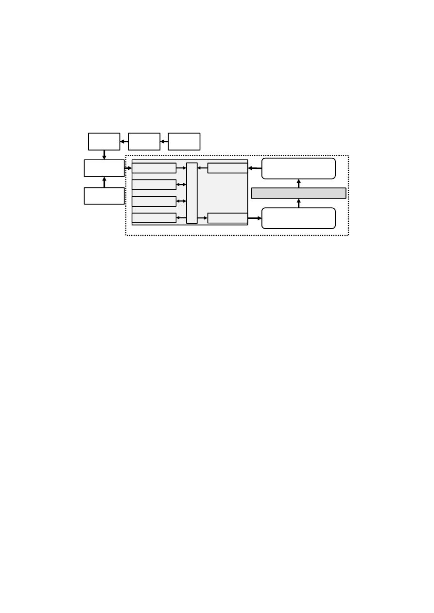
Figure 1. Flow chart of the optimization methodology based on the PGA algorithm and the toolkit of 
the SWMM model. 

2.1. Decision Variables   

The process of rehabilitation of a drainage network (Figure 1) involves modifying two types of 

DVs. On the one hand, there are variables related to pipe diameters, which seek to locate the best 
combination of sizes to obtain the minimum flooding. The optimization model analyzes the 
replacement of the pipes based on their transport capacity. The diameter may increase if the original 
pipe is insufficient to transport the flowing water or decrease if a hydraulic control device [25] 
should be installed to introduce the same head loss as the calculated pipe´s diameter. Consequently, 
the DV is the size of the pipes, and can vary from 0 (not replace) to a maximum value set before 
beginning the optimization process. Obviously, if the result associated with a pipe is 0, it is because 
it is not necessary to replace it for the correct operation of the network. Then, for a better 
understanding of the optimization methodology, it is convenient to define some parameters related 
to the pipes. So, N

C

 is the number of network conduits; m is the number of feasible conduits selected 

to be replaced, varying between 1 and N

C

; and ND is the number of candidate diameters, between 

ND

0

 and ND

max

.  

On the other hand, there are variables related to node storage capacity that seek the minimum 

volume of STs that reduce floods. The proposed methodology considers the possibility of installing 
an ST in each node of the network. This involves replacing an existing manhole with an 
underground ST. The land in which the rehabilitation of the drainage network is developed is 
mostly urban. Therefore, it is admitted that the depth of excavation is limited. Thus, the maximum 
depth of ST is what the manhole initially had, so the only parameter needed as DV is the ST cross 
section. Related to this, every node has a defined storage capacity related to its cross section and the 
model takes into account some nodes that could be modified into an ST. For this process, every node 
would have a DV representing the equivalent additional section corresponding to that of the STs in 
the case it would have been installed in the node location. The DV would vary between zero and a 
maximum value, predetermined before the optimization process and taking into account the 
restrictions of the urban geographical space of each node. If the nodes were not to be transformed 
into a tank, then the variable would have a value of 0, meaning that, it is not adequate to install a ST 

P
R

O

J

E
C
T

Input module

Runoff module

Routing module

Report module

Set Functions

Get Functions

Calibrated  

Network

Project 
rainfall 

Initial Data 

Network

Climate 

change

IDF Curve

Conduits: level 

Nodes: level &  flooding

PGA Genetic Algorithm

Pipes diameter

Size of STs

SWMM 

Simulator 

Toolkit

Simple optimization process

Figure 1.

Flow chart of the optimization methodology based on the PGA algorithm and the toolkit of

the SWMM model.

2.1. Decision Variables

The process of rehabilitation of a drainage network (Figure

1

) involves modifying two types

of DVs. On the one hand, there are variables related to pipe diameters, which seek to locate the
best combination of sizes to obtain the minimum flooding. The optimization model analyzes the
replacement of the pipes based on their transport capacity. The diameter may increase if the original

pipe is insufficient to transport the flowing water or decrease if a hydraulic control device [

25

] should

be installed to introduce the same head loss as the calculated pipe’s diameter. Consequently, the DV
is the size of the pipes, and can vary from 0 (not replace) to a maximum value set before beginning
the optimization process. Obviously, if the result associated with a pipe is 0, it is because it is not
necessary to replace it for the correct operation of the network. Then, for a better understanding of the
optimization methodology, it is convenient to define some parameters related to the pipes. So, N

C

is

the number of network conduits; m is the number of feasible conduits selected to be replaced, varying
between 1 and N

C

; and ND is the number of candidate diameters, between ND

0

and ND

max

.

On the other hand, there are variables related to node storage capacity that seek the minimum

volume of STs that reduce floods. The proposed methodology considers the possibility of installing an

ST in each node of the network. This involves replacing an existing manhole with an underground ST.

The land in which the rehabilitation of the drainage network is developed is mostly urban. Therefore, it

is admitted that the depth of excavation is limited. Thus, the maximum depth of ST is what the manhole
initially had, so the only parameter needed as DV is the ST cross section. Related to this, every node
has a defined storage capacity related to its cross section and the model takes into account some nodes
that could be modified into an ST. For this process, every node would have a DV representing the
equivalent additional section corresponding to that of the STs in the case it would have been installed
in the node location. The DV would vary between zero and a maximum value, predetermined before
the optimization process and taking into account the restrictions of the urban geographical space of
each node. If the nodes were not to be transformed into a tank, then the variable would have a value of
0, meaning that, it is not adequate to install a ST on the specific node’s location, maintaining thus the
initial storage capacity of the node. In case the initial hydraulic model has any type of water deposit,
the cross section of the deposit might be part of the optimization process.

Water 2019, 11, 515

6 of 22

For every node, whether it is regular or a storage node, its cross section S would be expressed

according to the following equation:

S

=

A

S

×

z

B

S

+

C

S

(1)

where A

S

, B

S

and C

S

are characteristic coefficients that adjust the tank’s section to different expressions,

and z is the water level of the node. In the case of considering tanks of constant section, A represents the
cross section while the coefficients B and C are null. However, considering tanks with variable section
does not imply a major difficulty in the problem implementation beyond choosing the right DVs.

Again, the definition of some parameters related to the nodes is important for the understanding

of the methodology. N

N

is the number of network nodes and n is the number of nodes selected to

potentially install a ST, varying between 1 and N

N

. Each node in which an ST can be installed has

the cross section (S) as DV. Since a heuristic optimization model is used, it is necessary to perform a
discretization of S. For this reason, a maximum value of the tank cross section (S

max

) is defined for

each node. In this way, N is the number of divisions in which S

max

is divided. Therefore, N determines

the resolution of the section S, varying between N

0

and N

max

. A simulation performed with the ST

cross section divided into N

0

parts is faster than a simulation performed N

max

divisions. So, to obtain

better calculation times, the number of divisions of the ST cross section could be reduced.

Additionally, to introduce tanks with a variable straight section does not imply major difficulty in

the problem implementation beyond choosing the right DVs.

As stated before, the size of the problem is a key aspect when trying to optimize real problems.

In this work, the optimization algorithm takes into consideration both pipes and nodes. The maximum
size of each rehabilitation scenario can be expressed by the following equation:

PS

max

=

N

C

ND

max

×

N

N

N

max

(2)

2.2. Objective Function

The objective function of the optimization problem is addressed in monetary units and is

represented as the sum of three cost functions:

•

The investment cost related to the substitution of each selected pipe of the network.

•

The investment cost linked to required volumes of STs to be installed in each solution.

•

The damage cost caused by the flooding level in various nodes of the network.

The mathematical expression of the objective function is given by Iglesias-Rey et al. [

26

]:

F

=

λ

1

m

∑

i=1

C

(

D

N

(

i

)) ×

L

i

+

λ

2

n

∑

j=1

C

(

V

DR

(

j

)) +

λ

3

N

F

∑

k=1

C

(

V

I

(

k

))

(3)

In Equation (3), the first term represents the rehabilitation or replacement cost of the m considered

pipes in the network. The second term represents the construction or expansion cost of volume V

DR

(j)

of the n STs installed in the drainage network. This cost concerns the existing STs whose volume will
be expanded, and the network nodes where new STs will be installed. The third term represents the
total flood damages costs [

27

] caused by the N

F

nodes in which a certain flooding volume V

I

(i) appears.

All the terms of the objective function have a weight coefficient λ

i

, in order to prioritize one term

versus another. If λ

i

is minimum (eventually null) the term is not considered, but if λ

i

is greater, the

term is considered in the objective function.

2.2.1. Pipe Replacement Cost Functions

This function represents the cost of rehabilitation of those pipes that are replaced in the

optimization process, either because they have poor internal conditions or because they have
insufficient transport capacity. In this work, the proposed function is adjusted based on real data from

Water 2019, 11, 515

7 of 22

manufacturers, relating the u

nit

cost of the pipes with their diameter. Finally, the pipe substitution cost

is in the form of a second-grade polynomial:

C

(

D

N

) =

α

×

D

N

+

β

×

D

2

N

(4)

where α and β are coefficients that must be adjusted in each case considering the costs of the project.

2.2.2. Storm Tank Installation Cost Functions

This cost function links the associated investment to the installation of STs in the network.

The tanks are installed on-line, simply said in series with the pipes existing in the network.
The determination of this cost function is fundamental at the moment to establish the size of the

adequate tanks to install. The function defines the tank installation cost based on its storage volume.
Here, the idea is to build small and median tanks implying the increase of the storage capacity of the
network and the water flow travelling time through the network. The mathematical expression of the
cost function is:

C

(

V

DR

) =

A

+

B

×

V

C

DR

(5)

In this expression, C(V

DR

) is the cost associated with the installation of an ST of volume V

DR

and

A, B and C are coefficients that must be adjusted in each case according to the specifics of the project.

2.2.3. Flood Damage Cost functions

Representation of the flood cost function can be based on either total flooding volume or floods

based on either total flooding volume or flood level. The first option allows us to eliminate totally
the flood, but this option will need more investments. This total water volume can be obtained by
summing the flooding volume of each flooding node. The second option allows reducing the flood and
the cost of the flood depending on the flooding area. Lee and Kim [

27

] showed that flooding damage is

different from flooding volume and that it was necessary to create a resilience index based on flooding
damage because some subareas are immediately damaged by a certain amount of flooding while other
subareas are not. They represented flood damage costs as a function of the level reached by water.

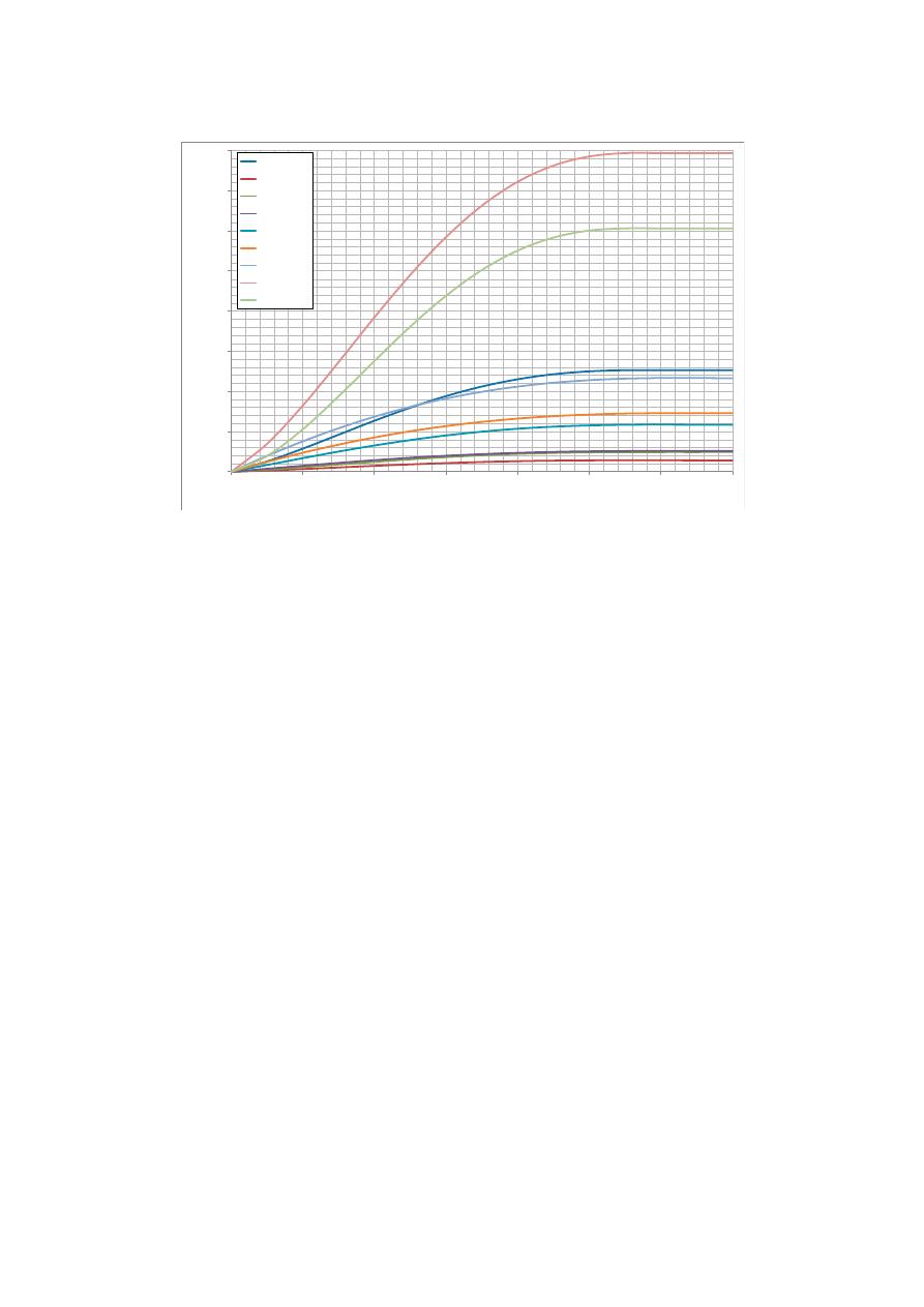
Using the Lee and Kim approach, flood damage costs have been determined for a drainage

network in Bogota (Colombia) analyzing the replacement costs of the damaged goods. A curve
representing the flood cost by m

2

of area as a function of the flood level was obtained for 6 different

social stratums, a commercial area and an industrial area [

23

]. There is also a curve representing the

average value of the study area. They can be observed in Figure

2

.

The formulation of the proposed problem considers that the resulting flood cost is defined

according to land use. Thus, the damage function is mathematically characterized by the expression:

C

(

y

) =

C

max

×

1

−

e

−λ

y

ymax

b

(6)

In this equation, C

max

represents the maximum cost, when flood level y

max

is reached. y is the

existing flood level in the specific node; λ = 4.89 and b = 2 are adjustment coefficients of the curve; and
the parameter y

max

= 1.4 is the level from which the maximal economic damage is produced. In all the

cases, Equation (6) depends totally on the value of C

max

, which is presented in Table

1

, for different

land uses and represents the maximum per area unit.

Table 1. C

max

values for different social strata (Str) linked to land uses.

Land Use

Str. 1

Str. 2

Str. 3

Str. 4

Str. 5

Str. 6

Commercial

Industrial Average

C

max

(

€/m

2

)

142

245

257

584

732

1168

3975

3041

1268

Water 2019, 11, 515

8 of 22

Water 2019, 10, x FOR PEER REVIEW   

8 of 23 

 

 

Figure 2. Flooding costs for different social strata linked to land uses. 

The formulation of the proposed problem considers that the resulting flood cost is defined 

according to land use. Thus, the damage function is mathematically characterized by the expression:   

𝐶(𝑦) = 𝐶

× 1 − 𝑒

 

 

(6)

 

In this equation, C

max

 represents the maximum cost, when flood level y

max 

is reached. y is the 

existing flood level in the specific node; λ = 4.89 and b = 2 are adjustment coefficients of the curve; 
and the parameter y

max

 = 1.4 is the level from which the maximal economic damage is produced. In 

all the cases, Equation (6) depends totally on the value of C

max

, which is presented in Table 1, for 

different land uses and represents the maximum per area unit.   

Table 1.  𝐶

 values for different social strata (Str) linked to land uses 

Land Use 

Str. 1 

Str. 2 

Str. 3 

Str. 4 

Str. 5 

Str. 6 

Commercial 

Industrial 

Average 

C

max

 (€/m

2

) 

142 245 257 584 732 1168  3975 

3041 

1268 

The cost evaluation C(y) described in Equation (6) required the determination of the flood level 

in each node. Therefore, the SWMM's ponded area model is used. This model assumes the definition 
of a ponded area (A

f

) in each node. In this way, the flood level is obtained as the relation between the 

flood volume V

f

 and the area A

f

.  

3. Methodology 

The optimal design or rehabilitation in drainage networks involves the search for solutions in 

very large spaces. Accordingly, the probability of finding minimum solutions is very small due to 
the immensity of SS and the existence of multiple local minima. Developments in the field of genetic 
algorithms (GAs) have proven to be useful in the optimization of drainage networks. 

The GAs test the evolution of a random population via a parallelism that is similar to Darwin´s 

law of natural selection. Some calibration parameters, including crossover probability, mutation 
probability and the population size control the optimization process. In this sense, the performance 
of population-based algorithms is directly related to the balance of exploration and exploitation of 
the SS. Traditionally, small population sizes have been related to premature convergence, since the 
population of the algorithm loses diversity too early, converging too early with poor solutions. 

0

500

1000

1500

2000

2500

3000

3500

4000

0

0.2

0.4

0.6

0.8

1

1.2

1.4

Fl

o

o

d

ing

 co

st

 (€

/m

2

)

Water level (m)

Average

Stratum 1

Stratum 2

Stratum 3

Stratum 4

Stratum 5

Stratum 6

Commercial

Industrial

Figure 2.

Flooding costs for different social strata linked to land uses.

The cost evaluation C(y) described in Equation (6) required the determination of the flood level in

each node. Therefore, the SWMM’s ponded area model is used. This model assumes the definition of a

ponded area (A

f

) in each node. In this way, the flood level is obtained as the relation between the flood

volume V

f

and the area A

f

.

3. Methodology

The optimal design or rehabilitation in drainage networks involves the search for solutions in

very large spaces. Accordingly, the probability of finding minimum solutions is very small due to

the immensity of SS and the existence of multiple local minima. Developments in the field of genetic
algorithms (GAs) have proven to be useful in the optimization of drainage networks.

The GAs test the evolution of a random population via a parallelism that is similar to Darwin´s

law of natural selection. Some calibration parameters, including crossover probability, mutation

probability and the population size control the optimization process. In this sense, the performance of
population-based algorithms is directly related to the balance of exploration and exploitation of the SS.
Traditionally, small population sizes have been related to premature convergence, since the population

of the algorithm loses diversity too early, converging too early with poor solutions. Conversely,
larger population sizes help ensure diversity of individuals, avoiding premature convergence, but the
algorithm might waste considerable time exploring regions of the SS without any kind of interest.
Consequently, parameter choice should be a trade-off between solution quality and search time.
It should be noted that this work uses a modified version of classical GA, PGA, whose complete
description can be found in [

18

].

In the same manner, the stopping criterion is important for population-based algorithms as

GAs. Three genetic algorithm stopping conditions are usually found in the literature: the objective
function value reaches a certain pre-defined value, a defined absolute number of generations are

performed or there is no improvement in the population for X iterations. In this work, the third option
was used, i.e., a maximal number of generations G without a change in the objective function value.

Considering the characteristics of the problem and based on previous experiences [

25

], a stopping

criterion of 1000 generations without change was selected. As in the calibration of the population size,
the choice of stopping criteria must prevent premature convergence, guaranteeing a good exploration
and exploitation of the SS.

Water 2019, 11, 515

9 of 22

Additionally, it should be noted that the DVs had to be discretized. On one hand, for STs a

maximum area is used, which is a function of the available surface with minimal urban impact and
divided into partitions. Therefore, STs can be discretized in N divisions (N = N

0

, . . . ,N

max

). On the

other hand, the number of candidate pipe diameters was ND (ND = ND

0

, . . . ,ND

max

).

As a previous step, some algorithm tests were performed considering the full SS, i.e., all the

nodes and lines of the network. According to protocol, several tests were carried out, in which it

was appreciated that the space of solutions is so large that the algorithm barely finds good solutions.
The enormous amount of local minimums causes the algorithm to be lost. A smaller solution space

allows the optimization algorithm to find minimum values more easily.

So, this work presents a methodology for the rehabilitation of large drainage networks, reducing

the SS of the problem. Additionally, this SS reduction will improve the solutions found by the PGA

when the entire SS was used. The different options to reduce the SS are the following:

•

Reduce the number of nodes (n) in which STs could potentially be installed.

•

Reduce the number of lines (m) in which there could potentially be a change in diameter.

•

Reduce the discretization N that is made of the section of each of the STs.

•

Reduce the number of candidate diameters ND in the pipes.

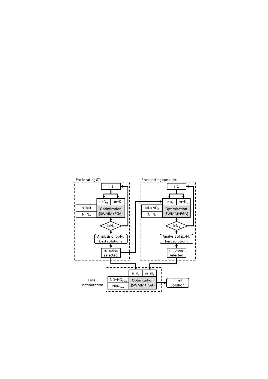
The four ways to reduce the SS have been organized in a specific methodology. The complete

process is summarized in Figure

3

, and basically consists of three stages: the pre-location of STs,

the pre-selection of conduits and the final optimization. In the following subsections, each of these
stages is described in detail.

Water 2019, 10, x FOR PEER REVIEW   

10 of 23 

 

   

Figure 3. Block diagram of the proposed methodology. 

3.1. Pre-locating Storm Tanks   

There are some previous studies oriented to the pre-locating of STs [25]. However, in this case 

methodology described in Figure 1 is used as a basic tool to determine the possible locations of the 
STs. The first step of the methodology is summarized on the left hand side of Figure 3. Some runs 
(N

it

) are performed with all the nodes of the network (n = N

N

), but without including the diameters 

in the optimization process (m = 0). Thus, N

it

 optimizations are made, considering only the cross 

section (S) of the tanks as DVs and without modifying the diameters of the network. Since the 
objective is the reduction of the SS, the discretization of the cross sections of the tanks (S) is carried 
out with the smallest number of divisions (N = N

0

). This coarse discretization of each section is 

carried out since the objective is not to calculate its exact value, but to determine in which nodes the 
installation of an ST is adequate. That is, the objective of this step is selecting the nodes where STs 
could be installed in the rehabilitation of the network, i.e., a pre-location of STs. 

In this step, the obtained solutions of initial trial runs are ranked according the value of the 

objective function. Each of these solutions contains a distribution of STs in the network and a 
dimensioning, even if approximate, of the ST size required in each node. However, the analysis is 
not focused on the size of the STs but on their location. Therefore, a percentage p

n

 of the best 

simulations is selected. The analysis of these simulations allows identifying the nodes where an ST 
could be installed and a list of n

s

 possible locations is created. These nodes are selected because they 

are repeated as the location of an ST in all the p

n

 selected solutions.   

3.2. Locating Lines of Possible Pipe Substitutions   

The objective of this second step is to reduce the number of pipes in which the diameter can be 

modified. Another set of N

it

 optimizations is run. The DVs of each optimization are the cross section 

of the n

s

 selected nodes in the previous process and the N

c

 conduits of the network. For both types 

of variables the reduction of the SS is applied. Therefore, the discretization of the cross section of 
the tanks is the coarsest (N = N

0

) and the range of pipes available is the smallest (ND = ND

0

). In this 

step, the aim is to find a pre-location of pipes to be substituted.   

Analogous to what happened in the previous step, an analysis of the solutions with the best 

value of the objective function is carried out. This analysis is not focused on the section of the tanks 

Figure 3.

Block diagram of the proposed methodology.

3.1. Pre-locating Storm Tanks

There are some previous studies oriented to the pre-locating of STs [

25

]. However, in this case

methodology described in Figure

1

is used as a basic tool to determine the possible locations of the

STs. The first step of the methodology is summarized on the left hand side of Figure

3

. Some runs (N

it

)

are performed with all the nodes of the network (n = N

N

), but without including the diameters in the

optimization process (m = 0). Thus, N

it

optimizations are made, considering only the cross section

Water 2019, 11, 515

10 of 22

(S) of the tanks as DVs and without modifying the diameters of the network. Since the objective is

the reduction of the SS, the discretization of the cross sections of the tanks (S) is carried out with the
smallest number of divisions (N = N

0

). This coarse discretization of each section is carried out since

the objective is not to calculate its exact value, but to determine in which nodes the installation of an
ST is adequate. That is, the objective of this step is selecting the nodes where STs could be installed in
the rehabilitation of the network, i.e., a pre-location of STs.

In this step, the obtained solutions of initial trial runs are ranked according the value of the

objective function. Each of these solutions contains a distribution of STs in the network and a
dimensioning, even if approximate, of the ST size required in each node. However, the analysis
is not focused on the size of the STs but on their location. Therefore, a percentage p

n

of the best

simulations is selected. The analysis of these simulations allows identifying the nodes where an ST
could be installed and a list of n

s

possible locations is created. These nodes are selected because they

are repeated as the location of an ST in all the p

n

selected solutions.

3.2. Locating Lines of Possible Pipe Substitutions

The objective of this second step is to reduce the number of pipes in which the diameter can be

modified. Another set of N

it

optimizations is run. The DVs of each optimization are the cross section

of the n

s

selected nodes in the previous process and the N

c

conduits of the network. For both types

of variables the reduction of the SS is applied. Therefore, the discretization of the cross section of the
tanks is the coarsest (N = N

0

) and the range of pipes available is the smallest (ND = ND

0

). In this step,

the aim is to find a pre-location of pipes to be substituted.

Analogous to what happened in the previous step, an analysis of the solutions with the best value

of the objective function is carried out. This analysis is not focused on the section of the tanks or on the
diameter of the ducts. The analysis is centered on locating the conduits whose dimensions have been
modified with respect to the initial situation.

Finally, a percentage p

m

of the best solutions are selected. The conduits selected are those that

appear repeated in the solutions defined by the percentage p

m

. Analyzing these solutions, the list of

m

s

pipes whose replacement is repeated in the p

m

best solutions is selected.

3.3. Final Optimization, Location and Optimization of Storm Tanks and Pipe Diameters

The last step considers the results of the two previous steps: the pre-location of the STs and the

location of the pipes that could potentially be rehabilitated. A simulation is defined with the n

s

selected

nodes and the m

s

selected lines. Although the number of DVs is smaller, the exploration of each of

these variables must now be greater. Therefore, the STs are discretized to the maximum (N = N

max

)

and the list of candidate diameters for the conduits is also the largest (ND = ND

max

). This final

optimization determines the location and size of the STs to be installed and the diameters of the pipes
to be rehabilitated.

In short, the reduction of SS in a problem with continuous and discrete variables has been based

on two aspects: the reduction of the number of DVs and the level of detail of each of the variables.
During the first two stages, the number of DVs is reduced by two with a lower level of exploration of
each variable. In the final simulation, a smaller number of variables is used, but with a higher level of
exploration. This reduction of the SS allows obtaining solutions to problems with large SS and multiple
local minimums.

4. Case Study

The drainage network is called E-Chicó. It is divided into 35 hydrological sub-catchments over

an area of 51 hectares. All the conduits are circular with diameters between 300 and 1400 mm, with a
total length around 5000 m. The network works completely by gravity with a maximum difference of
39.28 m.

Water 2019, 11, 515

11 of 22

The diagnosis of the network and the evaluation of the possible solutions have been carried

out using projected rain obtained by means of the alternative blocks method and the IDF curve.

This process has been done with the original IDF curve (actual rain), the one with which the network
was designed, and the one obtained after applying several climate change models [

22

]. As can be seen

(Figure

4

), the consideration of the climate change effects on the study area implies an increase in the

intensity of rainfall above 45%.

Water 2019, 10, x FOR PEER REVIEW   

11 of 23 

 

or on the diameter of the ducts. The analysis is centered on locating the conduits whose dimensions 
have been modified with respect to the initial situation.   

Finally, a percentage p

m

 of the best solutions are selected. The conduits selected are those that 

appear repeated in the solutions defined by the percentage p

m

. Analyzing these solutions, the list of 

m

s

 pipes whose replacement is repeated in the p

m

 best solutions is selected. 

3.3. Final Optimization, Location and Optimization of Storm Tanks and Pipe Diameters   

The last step considers the results of the two previous steps: the pre-location of the STs and the 

location of the pipes that could potentially be rehabilitated. A simulation is defined with the n

s

 

selected nodes and the m

s

 selected lines. Although the number of DVs is smaller, the exploration of 

each of these variables must now be greater. Therefore, the STs are discretized to the maximum (N = 
N

max

) and the list of candidate diameters for the conduits is also the largest (ND = ND

max

). This final 

optimization determines the location and size of the STs to be installed and the diameters of the 
pipes to be rehabilitated.   

In short, the reduction of SS in a problem with continuous and discrete variables has been 

based on two aspects: the reduction of the number of DVs and the level of detail of each of the 
variables. During the first two stages, the number of DVs is reduced by two with a lower level of 
exploration of each variable. In the final simulation, a smaller number of variables is used, but with 
a higher level of exploration. This reduction of the SS allows obtaining solutions to problems with 
large SS and multiple local minimums.   

4. Case Study 

The drainage network is called E-Chicó. It is divided into 35 hydrological sub-catchments over 

an area of 51 hectares. All the conduits are circular with diameters between 300 and 1400 mm, with a 
total length around 5000 meters. The network works completely by gravity with a maximum 
difference of 39.28 meters.   

The diagnosis of the network and the evaluation of the possible solutions have been carried out 

using projected rain obtained by means of the alternative blocks method and the IDF curve. This 
process has been done with the original IDF curve (actual rain), the one with which the network was 
designed, and the one obtained after applying several climate change models [22]. As can be seen 
(Figure 4), the consideration of the climate change effects on the study area implies an increase in the 
intensity of rainfall above 45%.   

 

Figure 4. Alternates blocks rains: Actual and Climate Change. 

The results of the first simulation considering the current IDF curve barely cause flooding in 

any node of the network. On the other hand, if the network is analyzed with the IDF curve obtained 
from climate change analysis, flooding occurs in 11 nodes of the network with a volume of 3833 m

3

, 

Figure 4.

Alternates blocks rains: Actual and Climate Change.

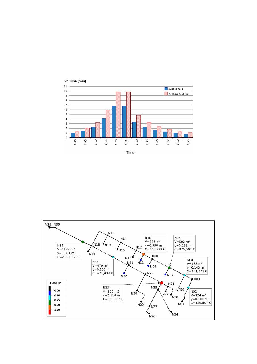
The results of the first simulation considering the current IDF curve barely cause flooding in

any node of the network. On the other hand, if the network is analyzed with the IDF curve obtained
from climate change analysis, flooding occurs in 11 nodes of the network with a volume of 3833 m

3

,

representing 18% of the total runoff of the network (21,233 m

3

). Figure

5

shows the nodes in which

the main floods occur (flood level over 10 cm), indicating the flood volume V; the maximum level y
reached by the water in the node and the cost associated with flood damage. Table

2

shows the detail

of the flooded nodes: the flood volume, area and level, and the damage cost obtained from Equation

(6). The nodes shown in Figure

5

are highlighted in bold in Table

2

.

Water 2019, 10, x FOR PEER REVIEW   

12 of 23 

 

representing 18% of the total runoff of the network (21,233 m

3

). Figure 5 shows the nodes in which 

the main floods occur (flood level over 10 cm), indicating the flood volume V; the maximum level y 
reached by the water in the node and the cost associated with flood damage. Table 2 shows the detail 
of the flooded nodes: the flood volume, area and level, and the damage cost obtained from Equation 
(6). The nodes shown in Figure 5 are highlighted in bold in Table 2.   

 

Figure 5. Representation of E-Chicó Flooding Nodes during the rainfall event. 

 

 

Figure 5.

Representation of E-Chicó Flooding Nodes during the rainfall event.

Water 2019, 11, 515

12 of 22

Table 2.

Data of the flooded nodes. .

Node.

Flood Volume (m

3

)

Flood Area (m

2

)

y

max

(m)

C(

€)

N02

123.56

1240

0.100

135,857

N04

132.56

930

0.143

181,375

N06

501.79

1890

0.265

875,502

N07

23.95

1250

0.019

6644

N09

1.82

1130

0.002

45

N10

385.12

700

0.550

646,838

N11

25.83

820

0.032

11,288

N23

949.54

450

2.110

569,922

N32

36.65

1500

0.024

12,727

N33

469.82

3030

0.155

671,908

N34

1181.87

3270

0.361

2,131,929

TOTAL

3832.51

5,244,034

The total cost of flood damage in the study area amounts to 5.24 million euros, which suggests

the importance of rehabilitating this sector of the network and applying the proposed methodology.

4.1. Application of the Drainage Network Rehabilitation Methodology to E Chico

In the first place, the validity of the methodology described in Figure

1

will be tested. Taking as a

starting point the simulation whose results are obtained in Figure

3

, three different simulation scenarios

are considered:

•

Scenario 1: Rehabilitation of the network based only on the modification of conduits of the
network and substituted them by another with different diameter. This scenario has 35 DVs, as all
the conduits are potentially changed.

•

Scenario 2: Rehabilitation of the network by installing only STs. This scenario also has 35 DVs,
corresponding to the 35 potential nodes in which STs can be installed. The maximum section to be
installed in the tank potentially installable is defined in each node. Subsequently, the optimization
method selects the cross section according to the discretization (N) of this variable. It should be
noted that the section minimum value corresponds to a diameter of 1.2 meters, corresponding to
the cross-sectional value of a manhole.

•

Scenario 3: Rehabilitation of the network combining the installation of conduits and STs.

The number of DVs is 70.

In order to be able to simulate the previous scenarios, all the data described in the formulation

of the problem should be defined. That is, it is necessary to specify the values of the installation
cost functions of the new conduits and the investment cost for the construction of the new STs to be
installed at the nodes. This involves determining the values of the parameters α and β of Equation (4)
and parameters A, B and C of Equation (5). In this case, price databases have been used for the area

where the network is located (Colombia). In this way, the values of the characteristic parameters of

Equations (4) and (5) are shown in Table

3

.

Table 3.

Coefficients for pipes and STs cost curves.

α

B

A

B

C

40.69

208.06

16923

318.4

0.65

At the same time, simulation of scenarios 1 and 3 requires defining a full range of pipe diameters.

The full range of diameters used in this case is shown in Table

4

. This table assumes a value of the

parameter ND = ND

max

= 25, since it must be combined with an additional state corresponding to

the event of leaving the drainage line as it is in the model; that is, without rehabilitation. Table

4

also

Water 2019, 11, 515

13 of 22

shows the installation cost of each diameter. These costs are obtained from the application of Equation

(4) with the coefficients defined in Table

3

.

Table 4.

Full range (ND = ND

max

) of commercial diameters used in the example.

D (mm)

300

350

400

450

500

600

700

800

900

1000

1100

1200

C (

€/m)

30.93

39.73

49.56

60.44

72.36

99.31

130.43

165.71

205.15

248.75

296.51

348.43

D (mm)

1300

1400

1500

1600

1800

1900

2000

2200

2400

2600

2800

3000

C (

€/m)

404.51

464.76

529.16

597.73

747.35

828.4

913.61

1096.52 1296.07 1512.27 1745.11 1994.6

The results of the optimization of the first three scenarios will allow comparing the effect of

carrying out the rehabilitation of the drainage network by different methods. The results will show the
benefits of rehabilitation through the combined use of STs and the replacement of pipes. One of the
main conclusions obtained from this first analysis is the time necessary to complete the simulations due
to the high number of DVs and the wide of solutions space. In addition, after performing numerous
simulations, a large dispersion in the results was also observed. Additionally, it could be concluded
that the combination of diameter changes and ST installation gave better results than the optimization
of any of them separately.

For the Scenario 3 corresponding to the rehabilitation of the whole network, some previous

simulations have been performed with the following characteristics: n = 35, m = 35, N = 40 and
ND = 25. The best objective function value obtained was 268,292

€, corresponding to the substitution

of 21 pipes and the installation of 16 STs. Afterwards, a sensitivity analysis with different population
sizes and different maximum number of generations was done, but no improvement was obtained.

So, the presented methodology has undergone an improvement process in order to obtain optimal

results without the need to significantly modify the parameters of the genetic algorithm used to

perform the simulations. Since these parameters are estimated based on the number of DVs and the

complexity of the problem, the objective was now focused on reducing the number of nodes and lines
that can be modified.

4.2. Application of the Solution Space Reduction Methodology to E-Chicó

The application of the proposed methodology (Figure

3

) to the E-Chicó network begins with the

process of pre-locating STs. The parameters used in this process are:

•

The number of simulations defined is one hundred (N

it

= 100).

•

The discretization of the ST area is reduced to its minimum value (N = N

0

= 10).

•

Only the sections of the tanks potentially to be installed in the nodes of the network are considered
as DVs (n = N

N

= 35).

•

No conduit can be modified during the process (m = 0).

•

The basic parameters of the PGA algorithm, population size (N

pop

) and the end criterion based on

a number of generations (N

gen

) without change, are fixed at 100.

Once all the simulations have been carried out, the percentage p

n

of solutions with the best value

in the objective function is selected. In short, the 10 best solutions are selected. In each one, it is
analyzed in which nodes an ST is installed. This generates a list of pre-locations of STs in the network.
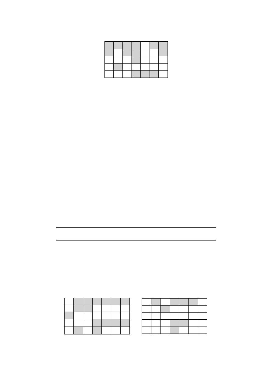
In this case, this list contains a total of 15 possible locations of the STs. In Figure

6

, the shaded cells

represent the selected nodes.

Water 2019, 11, 515

14 of 22

Water 2019, 10, x FOR PEER REVIEW   

14 of 23 

 

rehabilitation. Table 4 also shows the installation cost of each diameter. These costs are obtained 
from the application of Equation (4) with the coefficients defined in Table 3. 

Table 4. Full range (ND = ND

max

) of commercial diameters used in the example. 

D (mm) 

300 350 400 450 500 600 700  800  900  1000 1100 1200 

C (€/m) 

30.93 39.73 49.56 60.44 72.36 99.31 130.43 165.71 205.15 248.75 296.51 348.43 

D (mm) 

1300 1400 1500 1600 1800 1900 2000  2200  2400  2600  2800  3000 

C (€/m)  404.51 464.76 529.16 597.73 747.35 828.4 913.61 1096.52 1296.07 1512.27 1745.11 1994.6 

The results of the optimization of the first three scenarios will allow comparing the effect of 

carrying out the rehabilitation of the drainage network by different methods. The results will show 
the benefits of rehabilitation through the combined use of STs and the replacement of pipes. One of 
the main conclusions obtained from this first analysis is the time necessary to complete the 
simulations due to the high number of DVs and the wide of solutions space. In addition, after 
performing numerous simulations, a large dispersion in the results was also observed. Additionally, 
it could be concluded that the combination of diameter changes and ST installation gave better 
results than the optimization of any of them separately.   

For the Scenario 3 corresponding to the rehabilitation of the whole network, some previous 

simulations have been performed with the following characteristics: n = 35, m = 35, N = 40 and ND = 
25. The best objective function value obtained was 268,292 €, corresponding to the substitution of 21 
pipes and the installation of 16 STs. Afterwards, a sensitivity analysis with different population sizes 
and different maximum number of generations was done, but no improvement was obtained.   

So, the presented methodology has undergone an improvement process in order to obtain 

optimal results without the need to significantly modify the parameters of the genetic algorithm 
used to perform the simulations. Since these parameters are estimated based on the number of DVs 
and the complexity of the problem, the objective was now focused on reducing the number of nodes 
and lines that can be modified.   

4.2. Application of the Solution Space Reduction Methodology to E-Chicó   

The application of the proposed methodology (Figure 3) to the E-Chicó network begins with the 

process of pre-locating STs. The parameters used in this process are:   
•  The number of simulations defined is one hundred (N

it

 = 100).   

•  The discretization of the ST area is reduced to its minimum value (N = N

0

 = 10).   

•  Only the sections of the tanks potentially to be installed in the nodes of the network are 

considered as DVs (n = N

N

 = 35). 

•  No conduit can be modified during the process (m = 0).   
•  The basic parameters of the PGA algorithm, population size (N

pop

) and the end criterion based on 

a number of generations (N

gen

) without change, are fixed at 100.   

Once all the simulations have been carried out, the percentage p

n

 of solutions with the best 

value in the objective function is selected. In short, the 10 best solutions are selected. In each one, it 
is analyzed in which nodes an ST is installed. This generates a list of pre-locations of STs in the 
network. In this case, this list contains a total of 15 possible locations of the STs. In Figure 6, the 
shaded cells represent the selected nodes.   

 

Figure 6. Selected nodes as STs' pre-location. 

N01 N02 N03 N04 N05 N06 N07

N08 N09 N10 N11 N12 N13 N14

N15 N16 N17 N18 N19 N20 N21

N22 N23 N24 N25 N26 N27 N28

N29 N30 N31 N32 N33 N34 N35

Figure 6.

Selected nodes as STs’ pre-location.

In order to validate the methodology of pre-localization of STs, the previous process has been

repeated, but by expanding the discretization of the tank area to the maximum value (N = N

max

= 40).

The results obtained lead to the same list of selected nodes as indicated in Figure

6

.

The second stage of the SS reduction process is the pre-selection of conduits.

For this,

the pre-location of STs from the previous stage is used and a reduction in the number of potentially
substitutable pipes is sought. The parameters used in this process are:

•

The number of simulations is the same as in the previous stage (N

it

= 100).

•

The DVs are the areas of the ns nodes selected in the first stage and the diameters of all the
conduits (n = N

C

= 35) of the network.

•

The discretization of the area of the STs is kept at the minimum value, as it happened with the

previous stage of the process.

•

The basic parameters of the PGA algorithm are the same as in the previous phase (N

pop

= 100,

N

gen

= 100).

•

Instead of using the full range of diameters (Table

4

), a range of reduced diameters is used,

the details of which can be seen in Table

5

. This table shows the diameters D of the reduced range

and the unit costs (C) obtained from the application of the cost function (4) with the parameters of
the Table

3

. Note that although Table

5

only has 9 values, the number of options for the DV is

ND = 10. This additional value corresponds to the option of not taking any action on the pipe.

Table 5.

Reduced diameter range (ND = ND

0

= 10).

D (mm)

300

400

600

800

1000

1200

1500

1800

2000

C (

€/m)

30.93

49.56

99.31

165.7

248.74

348.43

529.16

747.35

913.61

Once the simulations have been carried out, it has been decided to define two different conduit

pre-selections. One is considering a probability of 10% of the best solutions (p

m1

= 10%) and another

one considering only 5% of solutions with a lower value of the objective function (p

m2

= 5%).

The preselected lines in each case are shown in Figure

7

. In the left part of the figure, the values

corresponding to 10% are collected, highlighting the preselected lines by gray color. On the right hand
side, the pipes selected for 5% of the best solutions obtained in this process are represented in an
analogous way.

Water 2019, 10, x FOR PEER REVIEW   

15 of 23 

 

In order to validate the methodology of pre-localization of STs, the previous process has been 

repeated, but by expanding the discretization of the tank area to the maximum value (N = N

max

 = 40). 

The results obtained lead to the same list of selected nodes as indicated in Figure 6.   

The second stage of the SS reduction process is the pre-selection of conduits. For this, the 

pre-location of STs from the previous stage is used and a reduction in the number of potentially 
substitutable pipes is sought. The parameters used in this process are:   
•  The number of simulations is the same as in the previous stage (N

it

 = 100). 

•  The DVs are the areas of the ns nodes selected in the first stage and the diameters of all the 

conduits (n =N

C

 = 35) of the network. 

•  The discretization of the area of the STs is kept at the minimum value, as it happened with the 

previous stage of the process.   

•  The basic parameters of the PGA algorithm are the same as in the previous phase (N

pop

 = 100, N

gen

 

= 100).   

•  Instead of using the full range of diameters (Table 4), a range of reduced diameters is used, the 

details of which can be seen in Table 5. This table shows the diameters D of the reduced range 
and the unit costs (C) obtained from the application of the cost function (4) with the parameters 
of the Table 3. Note that although Table 5 only has 9 values, the number of options for the DV is 
ND=10. This additional value corresponds to the option of not taking any action on the pipe.   

Table 5. Reduced diameter range (ND = ND

0

 = 10) 

D (mm) 

300  400  600  800  1000 1200 1500 1800 2000 

C (€/m) 

30.93 49.56 99.31 165.7 248.74 348.43 529.16 747.35 913.61 

Once the simulations have been carried out, it has been decided to define two different conduit 

pre-selections. One is considering a probability of 10% of the best solutions (p

m1

 = 10%) and another 

one considering only 5% of solutions with a lower value of the objective function (p

m2

 = 5%). The 

preselected lines in each case are shown in Figure  7.  In  the  left  part  of  the  figure,  the  values 
corresponding to 10% are collected, highlighting the preselected lines by gray color. On the right 
hand side, the pipes selected for 5% of the best solutions obtained in this process are represented in 
an analogous way.   

 

p

m1

 = 10% 

 

p

m2

 = 5% 

Figure 7. Selected lines to potentially be replaced for p

m1

 = 10% and p

m2

 = 5%. 

The pre-selection of ducts has been tested to validate performing the same simulations but 

using the full range of diameters (ND = ND

max

 = 25). The results obtained, in terms of the lines that 

would be pre-selected, are the same as those obtained in the case of using only the reduced range 
(ND = ND

0

 = 10).   

In short, the process of conduits pre-selection leads to select 15 pipes in case of selecting 10% of 

the best solutions or only 8 lines when the 5% of best simulations is considered. At this moment, the 
final stage of the process is the final optimization. In this phase, the reduction of the SS is used: 15 
possible locations of STs and 8 or 15 possible lines to be rehabilitated. Therefore, the analysis of the 
network requires the definition of two new scenarios:   
•  Scenario 4:  Rehabilitation of the network combining the possible installation of STs in the 15 

selected nodes and the 15 conduits that can be substituted.   

P01 P02 P03 P04 P05 P06 P07

P08 P09 P10 P11 P12 P13 P14

P15 P16 P17 P18 P19 P20 P21

P22 P23 P24 P25 P26 P27 P28

P29 P30 P31 P32 P33 P34 P35

P01 P02 P03 P04 P05 P06 P07

P08 P09 P10 P11 P12 P13 P14

P15 P16 P17 P18 P19 P20 P21

P22 P23 P24 P25 P26 P27 P28

P29 P30 P31 P32 P33 P34 P35

Figure 7.

Selected lines to potentially be replaced for p

m1

= 10% and p

m2

= 5%.

Water 2019, 11, 515

15 of 22

The pre-selection of ducts has been tested to validate performing the same simulations but

using the full range of diameters (ND = ND

max

= 25). The results obtained, in terms of the lines that

would be pre-selected, are the same as those obtained in the case of using only the reduced range
(ND = ND

0

= 10).

In short, the process of conduits pre-selection leads to select 15 pipes in case of selecting 10%

of the best solutions or only 8 lines when the 5% of best simulations is considered. At this moment,
the final stage of the process is the final optimization. In this phase, the reduction of the SS is used:

15 possible locations of STs and 8 or 15 possible lines to be rehabilitated. Therefore, the analysis of the

network requires the definition of two new scenarios:

•

Scenario 4: Rehabilitation of the network combining the possible installation of STs in the

15 selected nodes and the 15 conduits that can be substituted.

•

Scenario 5: It is the same scenario as the previous one (scenario 4), with the difference that the
number of potentially replaceable conduits is only 8.

4.3. Results Analysis

The results obtained from the optimization in the five scenarios considered are shown in Table

6

.

In each scenario, the following values appear: the number of DVs (nodes in which STs can potentially
be installed and lines where their diameter could potentially be modified), the value of the objective
function (divided into flood costs, investment costs in STs and investment costs in pipes), the number
of elements to install of each type (STs and conduits) and the size of the SS of the problem. The scenario
that offers the worst results (scenario 1) would be classic rehabilitation based solely on the replacement
of pipes. The solution based on the use of STs has better results than the rehabilitation based on pipe
substitution (scenario 2). However, the combined use of pipe substitution and installation of STs is
shown as the best option of all (scenario 3).

Table 6.

Result summary of the E Chico Optimization Process.

Scenario

No. DVs

Objective

Function

Terms in the Objective Function

No. Elements in the Solution

Nodes

Lines

Floods

STs

Pipes

STs

Pipes

1

0

35

791,214

24,753

0

766,461

0

21

2

35

0

273,455

5392

268,063

0

6

0

3

35

35

268,292

20,238

230,087

17,968

4

4

4

15

15

245,547

8353

213,133

24,061

4

5

5

15

8

213,981

12,701

186,353

14,927

3

3

Comparing the solutions that use joint rehabilitation pipes-STs, it is observed that the reduction of

the SS significantly improves the solutions. That is, pre-location of STs and pre-selection of conductions
reduce the SS in an amount that allows a better exploration. Therefore, according to Table

6

, the best

solution is the one proposed by scenario 5, which considers the installation of 3 STs and the replacement
of 3 conduits. As it is observed, the reduction of the SS between scenario 3 and scenarios 4 and 5 is
many orders of magnitude, which helps to explain the improvement in the solutions.

The methodology used assesses the flood economically. Therefore, the solutions of scenarios 4 and

5 present flood costs (8353 and 12,701 respectively). These flood costs correspond to nodes whose flood
level does not exceed 1.5 cm. However, from the point of view of the function defined in Equation

(6), any level of flooding has an associated cost. Additionally, Tables

7

and

8

present the results of the

flood nodes for scenarios 4 and 5. As can be seen, the cost of flooding is not zero. However, both flood

volumes (52.77 and 75.78 m

3

) and flood levels are very low. Therefore, from a practical point of view it

can be considered that the solutions are acceptable.

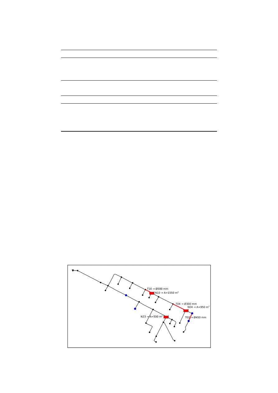
Water 2019, 11, 515

16 of 22

Table 7.

Flooding results in scenario 4.

Node

Flood Volume (m

3

)

Flood Area (m

2

)

y

max

(m)

C (

€)

N10

3.77

700

0.013

307.94

N32

12.96

1500

0.010

1680.29

N33

36.04

3030

0.009

6364.57

TOTAL

52.77

8352.80

Table 8.

Flooding results in scenario 5.

Node

Flood Volume (m

3

)

Flood Area (m

2

)

y

max

(m)

C (

€)

N02

12.82

1240

0.013

3024.66

N03

10.82

1080

0.010

1619.42

N32

12.96

1500

0.009

1681.56

N33

36.08

3030

0.012

6775.01

TOTAL

75.78

12,700.64

Figure

8

represents the location of the STs obtained in scenario 5, as well as their size. Also, the flooded

nodes are represented (blue nodes). Additionally, the figure represents the lines that have been necessary
to modify and the size of the new conduits. It should be noted that in the case of conduits T04 and T10,
the solution obtained involves the installation of a diameter smaller than the original one. This clearly
indicates the need to install in these sections a resistant element (a gate or an orifice) that introduces a
head loss equivalent to the one that involves the installation of the new smaller diameter.

The installation of control devices in drainage networks allows the accumulation of water in

certain points of the network, decreasing the time of concentration downstream, and thereby reducing
flooding. This is why this “hydraulic control” is one of the techniques that is often used to improve
the efficiency of STs. In this case, the appearance of solutions, such as those of conduits T04 and T10,
supposes the need to install a gate or an orifice at the outlet of the STs that introduces a certain head
loss. This head loss must be such that the equivalent capacity of the original pipeline together with the
control device used is equal to the transport capacity of the calculated pipeline.

In short, two of the three STs installed should have hydraulic control. Therefore, these tanks

must have a control element at the exit that contains the avenue of water in the tanks and reduces
the water travel time towards the downstream sections. If Figure

8

is compared with Figure

5

, the

installation of the STs together with the hydraulic control elements allows not only a reduction of
flooding upstream, but also control of flooding that occurred in nodes downstream from these STs (i.e.,
nodes N31 and N34).

Water 2019, 10, x FOR PEER REVIEW   

17 of 23 

 

Table 8. Flooding results in scenario 5. 

Node   Flood volume (m

3

) Flood area (m

2

) y

max

 (m) 

C (€) 

N02 

12.82 1240 

0.013 

3024.66 

N03 

10.82  

1080 

0.010 

1619.42 

N32 

12.96 1500 

0.009 

1681.56 

N33 

36.08 3030 

0.012 

6775.01 

TOTAL 

75.78  

12,700,64 

Figure 8 represents the location of the STs obtained in scenario 5, as well as their size. Also, the 

flooded nodes are represented (blue nodes). Additionally, the figure represents the lines that have 
been necessary to modify and the size of the new conduits. It should be noted that in the case of 
conduits T04 and T10, the solution obtained involves the installation of a diameter smaller than the 
original one. This clearly indicates the need to install in these sections a resistant element (a gate or 
an orifice) that introduces a head loss equivalent to the one that involves the installation of the new 
smaller diameter.   

The installation of control devices in drainage networks allows the accumulation of water in 

certain points of the network, decreasing the time of concentration downstream, and thereby 
reducing flooding. This is why this "hydraulic control" is one of the techniques that is often used to 
improve the efficiency of STs. In this case, the appearance of solutions, such as those of conduits T04 
and T10, supposes the need to install a gate or an orifice at the outlet of the STs that introduces a 
certain head loss. This head loss must be such that the equivalent capacity of the original pipeline 
together with the control device used is equal to the transport capacity of the calculated pipeline. 

In short, two of the three STs installed should have hydraulic control. Therefore, these tanks 

must have a control element at the exit that contains the avenue of water in the tanks and reduces the 
water travel time towards the downstream sections. If Figure 8 is compared with Figure 5, the 
installation of the STs together with the hydraulic control elements allows not only a reduction of 
flooding upstream, but also control of flooding that occurred in nodes downstream from these STs 
(i.e., nodes N31 and N34).   

 

Figure 8. Representation of STs installed and pipes to replace according to scenario 5 results. 

Simulations with a larger number of DVs are usually associated with a longer calculation time. 

However, the real difficulty of a problem is expressed by its size (PS

max

) according to Equation (2). 

Therefore, in Table 9 the size of the problem of each scenario is presented. The table also includes a 

Figure 8.

Representation of STs installed and pipes to replace according to scenario 5 results.

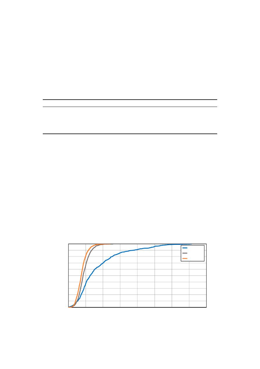
Water 2019, 11, 515

17 of 22

Simulations with a larger number of DVs are usually associated with a longer calculation time.

However, the real difficulty of a problem is expressed by its size (PS

max

) according to Equation (2).

Therefore, in Table

9

the size of the problem of each scenario is presented. The table also includes a

measurement of the calculation time, expressed as the number of times it is necessary to evaluate the
objective function.

As can be seen, the larger the size of the problem, the greater the number of evaluations of the

objective function required to find the solution. It is for this reason that the use of an SS reduction
technique and reduction of the size of the problem has been effective.

Table 9.

Size problem and computation time of the different scenarios.

Scenario

No. DVs

Problem Size

No. Evaluations of the Objective Function

1

35

4.0

×

10

38

51,200

2

35

5.8

×

10

61

65,485

3

70

2.3

×

10

100

709,000

4

30

2.8

×

10

76

205,300

5

23

4.1

×

10

69

151,300

The reduction in the number of DVs allows a better exploration of the SS, which means the smaller

the number of decision variables, the better the solution found. However, reducing the number of
DVs entails another effect. Simulations performed with large numbers of DVs cause a large dispersion
of solutions, while solutions obtained with fewer DVs offer a much narrower range of solutions.

Thus, Figure

9

represents a comparison of the solution variability range offered in scenarios 3, 4 and

5. It shows on the X-axis the relation between the value of the objective function in a simulation
and the minimum global value for this scenario. On the Y-axis is represented the frequency of the
different solutions obtained with respect to the minimum value obtained. That is, the more vertical
the curve, the greater concentration of solutions. On the contrary, if the slope of the curve is smaller,
it indicates that there is a greater dispersion of the solutions. Suppose that a value of 1.5 is set as a
reference (the solution obtained has a maximum extra cost of 50% over the optimal solution). In that
case, only 37% of the solutions obtained with scenario 3 are below that level. In the case of scenario 4,
66% of solutions present a cost smaller than 1.5 times the minimum value of the objective function.
For scenario 5, this percentage is even greater (81%). In short, the reduction of the SS not only allows
obtaining better solutions but at the same time it makes the range of good solutions (solutions close to
the minimum) greater.

Water 2019, 10, x FOR PEER REVIEW   

18 of 23 

 

measurement of the calculation time, expressed as the number of times it is necessary to evaluate the 
objective function.   

As can be seen, the larger the size of the problem, the greater the number of evaluations of the 

objective function required to find the solution. It is for this reason that the use of an SS reduction 
technique and reduction of the size of the problem has been effective. 

Table 9. Size problem and computation time of the different scenarios.

 

Scenario   No. DVs   

Problem 

Size  

No. Evaluations of the 

Objective function 

1 

35 

4.0 × 10

38

 51,200 

 

2 

35 

5.8 × 10

61

 65,485 

 

3 

70   

2.3 × 10

100

 709,000 

 

4 

30   

2.8 × 10

76

 205,300 

 

5 

23   

4.1 × 10

69

 151,300 

The reduction in the number of DVs allows a better exploration of the SS, which means the 

smaller the number of decision variables, the better the solution found. However, reducing the 
number of DVs entails another effect. Simulations performed with large numbers of DVs cause a 
large dispersion of solutions, while solutions obtained with fewer DVs offer a much narrower range 
of solutions. Thus, Figure 9 represents a comparison of the solution variability range offered in 
scenarios 3, 4 and 5. It shows on the X-axis the relation between the value of the objective function in 
a simulation and the minimum global value for this scenario. On the Y-axis is represented the 
frequency of the different solutions obtained with respect to the minimum value obtained. That is, 
the more vertical the curve, the greater concentration of solutions. On the contrary, if the slope of the 
curve is smaller, it indicates that there is a greater dispersion of the solutions. Suppose that a value of 
1.5 is set as a reference (the solution obtained has a maximum extra cost of 50% over the optimal 
solution). In that case, only 37% of the solutions obtained with scenario 3 are below that level. In the 
case of scenario 4, 66% of solutions present a cost smaller than 1.5 times the minimum value of the 
objective function. For scenario 5, this percentage is even greater (81%). In short, the reduction of the 
SS not only allows obtaining better solutions but at the same time it makes the range of good 
solutions (solutions close to the minimum) greater.   

   

Figure 9. Comparison between the whole problem results and methodology application results.

 

 

 

0%

10%

20%

30%

40%

50%

60%

70%

80%

90%

100%

1

1.5

2

2.5

3

3.5

4

4.5

5

Fr

equ

e

ncy

 (

%

)

Value of Objective Function / Minimum Value 

Scenario 3
Scenario 4
Scenario 5

Figure 9.

Comparison between the whole problem results and methodology application results.

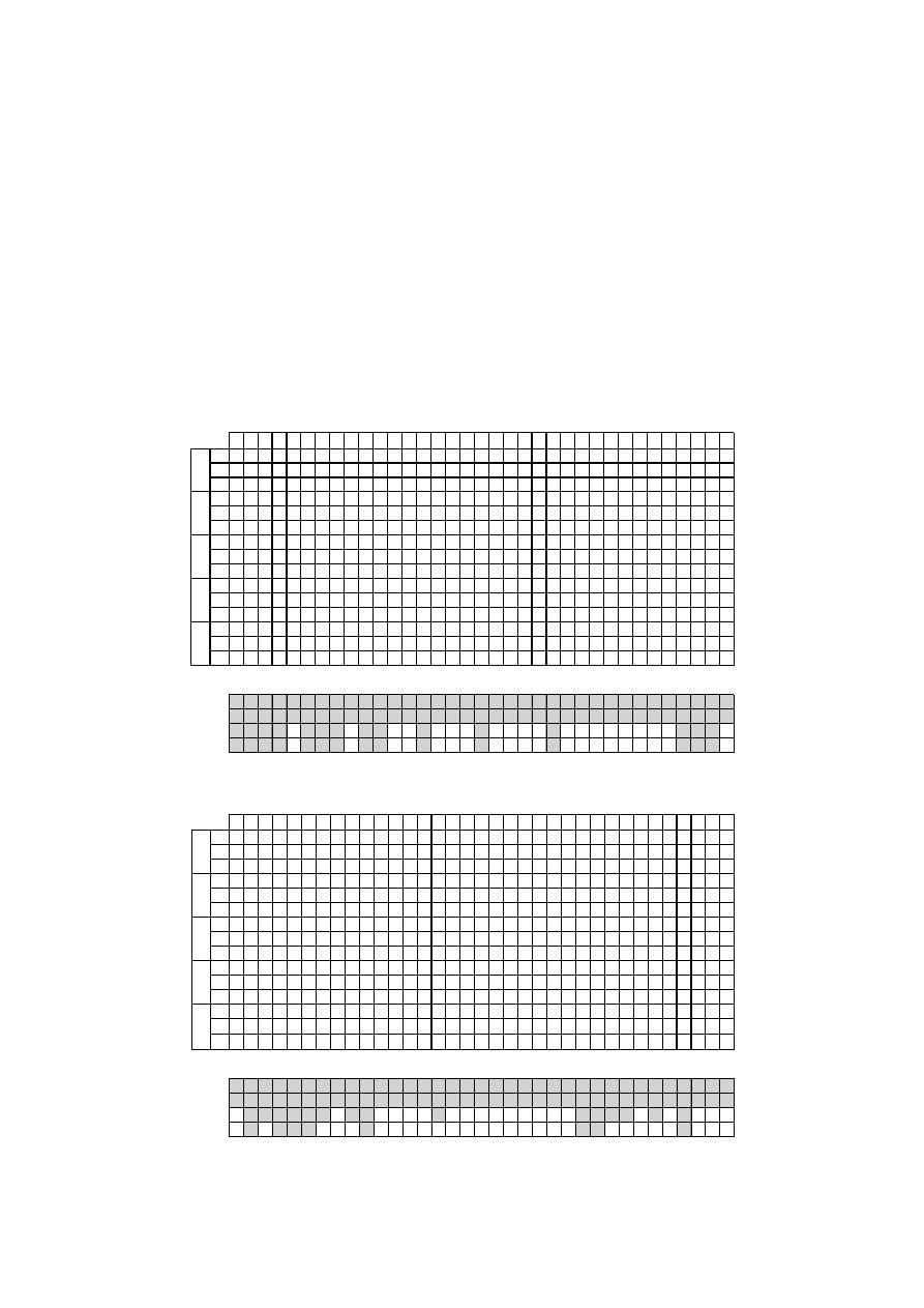
Water 2019, 11, 515

18 of 22

4.4. Sensitivity Analysis of the SS Reduction

The main uncertainty is whether the SS reduction methodology could affect the final solution. It

must be borne in mind that STs pre-localization and conduits pre-selection were performed using the
PGA algorithm with a population size N

pob

= 100 and a termination criterion N

gen

= 100. In order to

validate the selection, a sensitivity analysis of the selection process of STs and conduits has been carried

out. The process of reducing the SS was repeated with different values of N

pop

and N

gen

. The different

values of the population size were 35, 50, 75, 100 and 300 elements, while the values used as finalization

criteria were 50, 100 and 150 generations without a change in the value of the objective function. The
results obtained are shown in the following figures. In Figure

10

, the nodes that could potentially be a

ST location are collected for each combination of values of N

pop

and N

gen

. On the other hand, Figure

11

shows the lines potentially replaceable. In both cases, the node or line selected has been indicated with
an X in the corresponding cell.

Water 2019, 10, x FOR PEER REVIEW   

19 of 23 

 

4.4. Sensitivity Analysis of the SS Reduction   

The main uncertainty is whether the SS reduction methodology could affect the final solution. It 

must be borne in mind that STs pre-localization and conduits pre-selection were performed using 
the PGA algorithm with a population size N

pob

 = 100 and a termination criterion N

gen

 = 100. In order to 

validate the selection, a sensitivity analysis of the selection process of STs and conduits has been 
carried out. The process of reducing the SS was repeated with different values of N

pop

 and N

gen

. The 

different values of the population size were 35, 50, 75, 100 and 300 elements, while the values used as 
finalization criteria were 50, 100 and 150 generations without a change in the value of the objective 
function. The results obtained are shown in the following figures. In Figure 10, the nodes that could 
potentially be a ST location are collected for each combination of values of N

pop

 and N

gen

. On the other 

hand, Figure 11 shows the lines potentially replaceable. In both cases, the node or line selected has 
been indicated with an X in the corresponding cell. 

 

 

Figure 10. Sensitivity analysis results for pre-located STs with different N

pop

 and N

Gen

. 

 

Figure 11. Sensitivity analysis results for pre-selecting conduits with different N

pop

 and N

Gen

. 

N

pop

N

gen

1

2

3

4

5

6

7

8

9 10 11 12 13 14 15 16 17 18 19 20 21 22 23 24 25 26 27 28 29 30 31 32 33 34 35

50

X X X X X X

X X X X

X

X

X

X X X

X

100 X X X X

X X

X X X X

X

X

X

X X

X

150 X X X X X X X

X X X

X

X

X X X

50 X X X X X X X X

X X X X

X

X

X

X X

100 X X X X

X X X X X X X

X

X

X

X

150

X X X

X X X X X X X

X

X

X

50 X X

X X X X X X X X

X

X

X

X X X

100

X

X X X X X X X X

X

X

X

X X X

150 X X

X X X X X X X

X

X

X

X

50 X X X X

X X X X X X

X

X

X

X X X

100 X X X X

X X X

X X

X

X

X

X X X

150

X X X X X X X

X X

X

X

X

50

X X X

X X

X

X

X

X X

100

X

X

X X X

X X

X

X

150

X

X

X

X

X X

X

X

Scenario

X

X

X

X

X

X

X

X

X

X

X

X

X

X

X

X

X

3

4

5

2

50

75

100

300

Id of the nodes in which a storage structure is installed

35

N

pop

N

gen

1

2

3

4

5

6

7

8

9 10 11 12 13 14 15 16 17 18 19 20 21 22 23 24 25 26 27 28 29 30 31 32 33 34 35

50

X X X X X

X X

X X X X X

X

X

X

X

X X

100 X X X X X X X X X X X

X

X

X

150

X X X X X

X X

X

X

X

X

X

X

X

50

X X X

X X X X X X

X

X

X

X X

X

X

100

X X X

X X X X X X

X

X

X

150

X X X

X X X

X X X X

X

X

X X

X

X

50

X X X

X X X

X X X X

X

X

X

X X

X

X

100

X X X X X X X X X

X X

X

X

X

X

X

150

X X X X X X X X X

X X X

X

X

X

50

X X X X X X X X X X

X

X

X X

X

X

X

X

100

X X X

X X

X X X

X

X

150

X X X

X X X X X

X

X

X

X

X X

X

50

X X X

X

X X X X

X

X

X X

X

X

X

X

100

X X X

X X X X X X X X

X

X

X

X

150

X

X

X X X X X X

X

X X X X X

X X

X

Scenario

X X X

X

X X X

X

X X

X

X

X X X X X

X

X X X

X

X

X

X

X

X

X

X

X

X

X

X

Id of the conduit in which a storage structure is installed

1

3

4

5

300

35

50

75

100

Figure 10.

Sensitivity analysis results for pre-located STs with different N

pop

and N

Gen

.

Water 2019, 10, x FOR PEER REVIEW   

19 of 23 

 

4.4. Sensitivity Analysis of the SS Reduction   

The main uncertainty is whether the SS reduction methodology could affect the final solution. It 

must be borne in mind that STs pre-localization and conduits pre-selection were performed using 
the PGA algorithm with a population size N

pob

 = 100 and a termination criterion N

gen

 = 100. In order to 

validate the selection, a sensitivity analysis of the selection process of STs and conduits has been 
carried out. The process of reducing the SS was repeated with different values of N

pop

 and N

gen

. The 

different values of the population size were 35, 50, 75, 100 and 300 elements, while the values used as 
finalization criteria were 50, 100 and 150 generations without a change in the value of the objective 
function. The results obtained are shown in the following figures. In Figure 10, the nodes that could 
potentially be a ST location are collected for each combination of values of N

pop

 and N

gen

. On the other 

hand, Figure 11 shows the lines potentially replaceable. In both cases, the node or line selected has 
been indicated with an X in the corresponding cell. 

 

 

Figure 10. Sensitivity analysis results for pre-located STs with different N

pop

 and N

Gen

. 

 

Figure 11. Sensitivity analysis results for pre-selecting conduits with different N

pop

 and N

Gen

. 

N

pop

N

gen

1

2

3

4

5

6

7

8

9 10 11 12 13 14 15 16 17 18 19 20 21 22 23 24 25 26 27 28 29 30 31 32 33 34 35

50

X X X X X X

X X X X

X

X

X

X X X

X

100 X X X X

X X

X X X X

X

X

X

X X

X

150 X X X X X X X

X X X

X

X

X X X

50 X X X X X X X X

X X X X

X

X

X

X X

100 X X X X

X X X X X X X

X

X

X

X

150

X X X

X X X X X X X

X

X

X

50 X X

X X X X X X X X

X

X

X

X X X

100

X

X X X X X X X X

X

X

X

X X X

150 X X

X X X X X X X

X

X

X

X

50 X X X X

X X X X X X

X

X

X

X X X

100 X X X X

X X X

X X

X

X

X

X X X

150

X X X X X X X

X X

X

X

X

50

X X X

X X

X

X

X

X X

100

X

X

X X X

X X

X

X

150

X

X

X

X

X X

X

X

Scenario

X

X

X

X

X

X

X

X

X

X

X

X

X

X

X

X

X

3

4

5

2

50

75

100

300

Id of the nodes in which a storage structure is installed

35

N

pop

N

gen

1

2

3

4

5

6

7

8

9 10 11 12 13 14 15 16 17 18 19 20 21 22 23 24 25 26 27 28 29 30 31 32 33 34 35

50

X X X X X

X X

X X X X X

X

X

X

X

X X

100 X X X X X X X X X X X

X

X

X

150

X X X X X

X X

X

X

X

X

X

X

X

50

X X X

X X X X X X

X

X

X

X X

X

X

100

X X X

X X X X X X

X

X

X

150

X X X

X X X

X X X X

X

X

X X

X

X

50

X X X

X X X

X X X X

X

X

X

X X

X

X

100

X X X X X X X X X

X X

X

X

X

X

X

150

X X X X X X X X X

X X X

X

X

X

50

X X X X X X X X X X

X

X

X X

X

X

X

X

100

X X X

X X

X X X

X

X

150

X X X

X X X X X

X

X

X

X

X X

X

50

X X X

X

X X X X

X

X

X X

X

X

X

X

100

X X X

X X X X X X X X

X

X

X

X

150

X

X

X X X X X X

X

X X X X X

X X

X

Scenario

X X X

X

X X X

X

X X

X

X

X X X X X

X

X X X

X

X

X

X

X

X

X

X

X

X

X

X

Id of the conduit in which a storage structure is installed

1

3

4

5

300

35

50

75

100

Figure 11.

Sensitivity analysis results for pre-selecting conduits with different N

pop

and N

Gen

.

Water 2019, 11, 515

19 of 22

The sensitivity analysis of Figures

10

and

11

validates the SS reduction methodology based on the

pre-location of STs and the pre-selection of conduits. In the lower part of Figure

10

, the DVs used in

each scenario are indicated by a shaded cell, and X indicates the nodes that finally provide a solution
for the installation of a ST. The nodes that finally appear as solutions in the scenarios are those that
had been selected mostly in the process of pre-selection of STs. In short, regardless the value of N

pop

and N

gen

the preselected nodes would have been almost the same, and in any case those that appear in

the final solutions of scenarios 3, 4 and 5 would have always been selected.

Something similar happens in the case of pre-selection of conduits. Figure

11

shows the results

of the sensitivity analysis and the results of scenarios 1, 3, 4 and 5. As in Figure

10

, the DVs used are

indicated as shaded cells, and the lines that are finally replaced are indicated with an X. The results
show that the lines selected for different values of N

pop

and N

gen

are almost the same. That is, selected

lines are those that are finally found in the final solutions of scenarios 3, 4 and 5. Moreover, N

pop

and

N

gen

parameters have no influence on the pre-location of STs or on the pre-selection of pipes. Therefore,

the SS reduction methodology can be considered reliable.

5. Conclusions

The proposed methodology for the rehabilitation of drainage networks, based on the combined

use of STs and the replacement of conduits, has been shown to be effective in solving the problems
of insufficient drainage networks. Despite the effectiveness of the presented methodology, a certain
disparity is detected in the obtained solutions due to the enormous size of the SS. Therefore,
a complementary strategy that allows the reduction of SS is presented. Once the methodologies
area applied to the case study, it is possible to extract the following conclusions:

•

The increase in rainfall intensities caused by climate change causes originally well-designed
networks to present flooding problems. The use of STs has been shown as an effective technique to
solve this problem. However, the effectiveness of this method is even greater when it is combined

with the rehabilitation of some pipes of the drainage network. The results shown by scenarios 1,

2 and 3 presented above show how the combined action of STs and pipe renewal (scenario 3) is
much more effective than the isolated action of any of the other two actions (scenarios 1 and 2).

•

The number of DVs required for the rehabilitation of a drainage network can be very high.

This may cause (Figure

9

) the optimization model to give solutions that are quite dispersed

and sometimes far from the optimal values required. It is well known that the importance of
meta-heuristic algorithms does not lie in the optimality of their solutions, but in the ability to
obtain large sets of good solutions. That is why the disparity of solutions observed with large
numbers of DVs can become a problem.

•

An alternative methodology has been proposed for the reduction of the SS that permit us to
locate solutions that are better and less dispersed than those obtained with the initial model.

This methodology is based on the pre-location of STs and the pre-selection of possible conduits.
The methodology uses the PGA developed, reducing the SS by using a smaller discretization of

the size of the STs, a smaller range of diameters of pipes, and a smaller number of elements (tanks
and pipes). The final result has proven to be effective for the cases analyzed, not only because it
reduces SS and computing times, but also because it obtains better solutions (scenario 4 and 5).
Likewise, the solutions obtained with the scenarios that use a reduced SS (scenarios 4 and 5) are
much more concentrated and less dispersed (Figure

9

) than those obtained initially.

•

The SS reduction methodology in the case study has been shown to be reliable and stable since

variations in the N

pop

and N

gen

parameters of the PGA model hardly modify the preselected lines

and nodes.

Water 2019, 11, 515

20 of 22

The best solutions suggest the suitability of installing control devices as a strategy to improve the

operation of drainage networks. These control elements are static: either orifices or gates in a fixed

position. In the solutions of scenarios 4 and 5, the installation of STs is complemented with the presence

of this devices at the exit of the ST. This additional hydraulic resistance has been represented by a
conduit with a diameter lower than the original one. As indicated previously, this type of operation
helps to increase the concentration times in the critical nodes of the network.

The methodology based on the use of STs is adequate for the rehabilitation of drainage networks.

The optimization model and the SS reduction methodology allow obtaining good solutions to a really

complex problem. The resolution methodology used in the E-Chicó network can be extended to
any type of drainage network, since the approach of the method has been so general to be easily
extrapolated to other cases.

The extrapolation of the method to other networks generates some interesting uncertainties,

such as the possible behavior of drainage networks with pumping stations. In this case, where the
network has already installed pumping systems, the start and stop levels of the pumps and the size
of the suction tank can be defined as DV. In the case of installing new pumping systems, the DVs

would be the flows to be evacuated by each pump. In this case, it would be necessary to include in the

objective function the investment cost associated with the construction of the new pumping equipment.
In any case, it seems that the exposed methodology would be applicable to this situation.

It should be noted that the best solutions do not always eliminate the presence of floods in the

network. In the case that solutions without flood are desirable, there are two possibilities. The first
one is to allocate higher costs to the presence of floods that shift the optimum to solutions where the
installation of STs or new conduits is profitable. The second option would be to run the problem
statement from a multi-criteria point of view. With this type of approach, one could determine the
level of investment required for each level of expected flood damage.

Supplementary Materials:

The following are available online at

http://www.mdpi.com/2073-4441/11/3/515/

s1

.

Author Contributions:

All authors contributed extensively to the work presented in this paper. U.A.N.N P.L.I.-R.

and F.J.M. contributed to the research, the modeling, the data analysis, and the writing of the paper. D.M.-M.
contributed in the development of some cost functions and the manuscript review. J.G.S.V. collaborated to the
modeling part of the E-Chicó drainage network used in the case study.

Funding:

This research was funded by the Program Fondecyt Regular, grant number 1180660.

Acknowledgments:

This work was supported by the Program Fondecyt Regular (Project 1180660) of the Comision

Nacional de Investigación Científica y Tecnológica (Conicyt), Chile.

Conflicts of Interest:

The authors declare no conflict of interest.

Abbreviations

The following abbreviations are used in this manuscript:

DV

Decision variable

GA

Genetic Algorithm

IDF

Intensity, Duration, Frequency

NSGA

Non-dominated Sorting Genetic Algorithm

PGA

Pseudo-Genetic Algorithm

SS

Search Space, Solution Space

ST

Storm Tanks

SWMM

Storm Water Management Model

WTP

Wastewater Treatment Plant

Water 2019, 11, 515

21 of 22

Notation

α

, β

characteristic coefficients for the cost function related to the installation of new conduits

A, B

characteristic coefficients for the cost function related to the installation of a new ST of
volumen V

DR

A

f

ponded area of a node to represent the flood level

A

S

, B

S,

C

S

characteristic coefficients of tank cross section equation

b

adjusts coefficients of the damage cost curve

C(DN(i))

ccost related to the installation of the diameter i

C(V

DR

(j))

cost related to the construction or expansion of the volumen V

DR

(j)

C(y)

damage cost related to a flood level y

C

max

maximum economic damage cost, when flood level y

max

is reached

G

number of generations of the PGA

L

i

length of the conduit i

λ

adjusts coefficients of the damage cost curve

λ

i

Lagrange multipliers of the objective function

m

number of feasible conduits selected to be replaced, varying between 1 and N

C

m

s

number of possible pipe locations created after the pre-selecting pipes location step

n

number of nodes selected to potentially install a ST, varying between 1 and N

N

.

N

number of divisions for the cross section S, varying between N

0

and N

max

N

C

number of conduits of the network

N

D

number of candidate diameters, between ND

0

and ND

max

N

gen

stop criteria: maximal number of generations G without change in the objective function
value

N

it

number of optimizations (runs) of the PGA algorithm to develop one of the steps of the SS
reduction method

N

N

number of nodes of the network

N

pop

population size of the PGA

n

s

number of possible ST locations after the pre-locating STs step

p

m

percentage of the best solutions selected in the pre-selecting pipes location step

p

n

percentage of the best solutions selected in the pre-locating STs step

PS

max

maximum size of the optimization problem

S

tank’s cross section

S

max

maximum value of the tank cross section

V

DR

(j)

volume of the j-th ST

V

f

volume of water flooded in a node

y

existing flood level on the specific node

y

max

level from which the maximal economic damage is produced

z

water level in a storm tank

References

1.

Howard, C.D.D. Theory of Storage and Treatment-Plant Overflows. J. Environ. Eng. Div. 1976, 102, 709–722.

2.

di Toro, D.M.; Small, M.J. Stormwater Interception and Storage. J. Environ. Eng. Div. 1979, 105, 43–54.

3.

Loganathan, V.G.; Deniur, J.W.; Segarra, R.I. Planning Detention Storage for Stormwater Management.
J. Water Resour. Plan. Manag. 1985, 111, 382–398. [

CrossRef

]

4.

Meredith, D.D.; Middleton, A.C.; Smith, J.R. Design of Detention Basins for Industrial Sites. J. Water Resour.

Plan. Manag. 1990, 116, 586–591. [

CrossRef

]

5.

Takamatsu, M. Hydraulic model for sedimentation in storm-water detention basins. J. Environ. 2009, 136,
527–534. [

CrossRef

]

6.

de Martino, G.; de Paola, F.; Fontana, N.; Marini, G.; Ranucci, A. Pollution Reduction in Receivers:
Storm-Water Tanks. J. Urban Plan. Dev. 2011, 137, 29–38. [

CrossRef

]

7.

Li, Y.; Kang, J.-H.; Lau, S.-L.; Kayhanian, M.; Stenstrom, M.K. Optimization of Settling Tank Design to
Remove Particles and Metals. J. Environ. Eng. 2008, 134, 885–894. [

CrossRef

]

Water 2019, 11, 515

22 of 22

8.

Fu, G.; Butler, D.; Khu, S.T. Multiple objective optimal control of integrated urban wastewater systems.

Environ. Model. Softw. 2008, 23, 225–234. [

CrossRef

]

9.

Vanrolleghem, P.; Benedetti, L.; Meirlaen, J. Modelling and real-time control of the integrated urban

wastewater system. Environ. Model. Softw. 2005, 20, 427–442. [

CrossRef

]

10.

Andrés-Doménech, I.; Montanari, A.; Marco, J.B. Efficiency of Storm Detention Tanks for Urban Drainage
Systems under Climate Variability. J. Water Resour. Plan. Manag. 2012, 138, 36–46. [

CrossRef

]

11.

Butler, D.; Schütze, M. Integrating simulation models with a view to optimal control of urban wastewater
systems. Environ. Model. Softw. 2005, 20, 415–426. [

CrossRef

]

12.

Deb, K.; Pratap, A.; Agarwal, S.; Meyarivan, T. A fast and elitist multiobjective genetic algorithm: NSGA-II.
IEEE Trans. Evol. Comput. 2002, 6, 182–197. [

CrossRef

]

13.

Wang, M.; Sun, Y.; Sweetapple, C. Optimization of storage tank locations in an urban stormwater drainage
system using a two-stage approach. J. Environ. Manag. 2017, 204, 31–38. [

CrossRef

] [

PubMed

]

14.

Rossman, L.A. Storm Water Management Model User’s Manual; U.S. Environmental Protection Agency:
Cincinnati, OH, USA, 2015.

15.

Gaudio, R.; Penna, N.; Viteritti, V. A combined methodology for the hydraulic rehabilitation of urban
drainage networks. Urban Water J. 2016, 13, 644–656. [

CrossRef

]

16.

Sebti, A.; Bennis, S.; Fuamba, M. Cost Optimization of Hydraulic and Structural Rehabilitation of Urban
Drainage Network. J. Infrastruct. Syst. 2014, 20, 04014009. [

CrossRef

]

17.

Ugarelli, R.; di Federico, V. Optimal Scheduling of Replacement and Rehabilitation in Wastewater Pipeline
Networks. J. Water Resour. Plan. Manag. 2010, 136, 348–356. [

CrossRef

]

18.

Mora-Melia, D.; Iglesias-Rey, P.L.; Martinez-Solano, F.J.; Fuertes-Miquel, V.S. Design of Water Distribution
Networks using a Pseudo-Genetic Algorithm and Sensitivity of Genetic Operators. Water Resour. Manag.
2013

, 27, 4149–4162. [

CrossRef

]

19.

Martínez-Solano, F.J.; Iglesias-Rey, P.L.; Saldarriaga, J.G.; Vallejo, D. Creation of an SWMM Toolkit for Its

Application in Urban Drainage Networks Optimization. Water 2016, 8, 259. [

CrossRef

]

20.

Maier, H.R.; Kapelan, Z.; Kasprzyk, J.; Kollat, J.; Matott, L.S.; Cunha, M.C.; Dandy, G.C.; Gibbs, M.S.;
Keedwell, E.; Marchi, A.; et al. Evolutionary algorithms and other metaheuristics in water resources: Current
status, research challenges and future directions. Environ. Model. Softw. 2014, 62, 271–299. [

CrossRef

]

21.

Mala-Jetmarova, H.; Sultanova, N.; Savic, D. Lost in optimisation of water distribution systems? A literature
review of system operation. Environ. Model. Softw. 2017, 93, 209–254. [

CrossRef

]

22.

Gulizia, C.; Camilloni, I. Comparative analysis of the ability of a set of CMIP3 and CMIP5 global climate
models to represent precipitation in South America. Int. J. Climatol. 2015, 35, 583–595. [

CrossRef

]

23.

Cunha, M.C.; Zeferino, J.A.; Simões, N.E.; Saldarriaga, J.G. Optimal location and sizing of storage units in a
drainage system. Environ. Model. Softw. 2016, 83, 155–166. [

CrossRef

]

24.

Mora-Melia, D.; Iglesias-Rey, P.L.; Martinez-Solano, F.J.; Ballesteros-Pérez, P. Efficiency of Evolutionary

Algorithms in Water Network Pipe Sizing. Water Resour. Manag. 2015, 29, 4817–4831. [

CrossRef

]

25.

Leitão, J.P.; Carbajal, J.P.; Rieckermann, J.; Simões, N.E.; Marques, A.S.; de Sousa, L.M. Identifying the best
locations to install flow control devices in sewer networks to enable in-sewer storage. J. Hydrol. 2018, 556,
371–383. [

CrossRef

]

26.

Iglesias-Rey, P.L.; Martínez-Solano, F.J.; Saldarriaga, J.G.; Navarro-Planas, V.R. Pseudo-genetic Model
Optimization for Rehabilitation of Urban Storm-water Drainage Networks. Procedia Eng. 2017, 186, 617–625.
[

CrossRef

]

27.

Lee, E.; Kim, J. Development of Resilience Index Based on Flooding Damage in Urban Areas. Water 2017,
9, 428. [

CrossRef

]

© 2019 by the authors. Licensee MDPI, Basel, Switzerland. This article is an open access

article distributed under the terms and conditions of the Creative Commons Attribution

(CC BY) license (http://creativecommons.org/licenses/by/4.0/).