
AN ENERGY BASED METHODOLOGY APPLIED TO D-TOWN
Saldarriaga J.
1
, Páez D.
1
, Hernández D.
1
, Bohórquez J.
1
1
Universidad de los Andes
ABSTRACT
This paper presents a methodology to rehabilitate and design the expansion of D-Town water
distribution network. The methodology uses the Unitary Power concept, the OPUS design algorithm
and an optimization process for reducing pumps usage. The final result shows that all the
requirements of the problem were accomplished with a small computational effort as expected by
using energy based processes and criteria. Although both mentioned concepts were developed to
minimize constructive costs, the correlation between the constructive an operational costs with
GHG emissions, allows its minimization as well. On the other hand, the minimization of water age
couldn’t be considered as a main objective because of the nature of the used methodologies.
INTRODUCTION
A common problem regarding new water distribution system (WDS) designs is based on predicted
demands. The demands are found based on several assumptions, some of which does not occur and
therefore the system requires some modifications in its operation and configuration (i.e.
rehabilitation) in order to supply the requirements on the demand nodes, after the start of the
WDS’s operation. Taking into account that a WDS consists of several elements, accessories and
operational rules, the problem has many decision variables that define a wide larger solution space.
Therefore an optimization problem can be defined, with its correspondent restrictions, decision
variables and the objective functions being the operational and constructive costs, the water quality
and environmental impact, among others.
Some main problems related to water distribution systems, such as design, calibration, operation,
rehabilitation and else, are being solved using metaheuristic algorithms (e.g. Zecchin et al., 2006;
Reca et al., 2007; Geem, 2009). This implies that most of these methodologies require several
number of iterations, each of which require at least one hydraulic simulation and, therefore,
considerable computational time (especially for real networks). An alternative approach based on
the I Pai Wu (1975) concept of “Optimal Energy Gradient Line” (for drip irrigation main lines) has
been developed around the problems of design and operation (e.g. Villalba, 2004; Ochoa, 2009;
Saldarriaga et al., 2011). The major advantages of these methodologies are the significant reduction
of iterations and their deterministic character, in contrast to the stochastic one of metaheuristic
algorithms
The I Pai Wu concept is extended to looped networks by defining a Energy Surface as the surface
that represents the total energy (written as a hydraulic head) for each node in the network and
studying the shapes of that surface produced by optimal designs, looking for a pattern that allows
the estimation of the optimal surface for other networks. In this study that concept is applied to
solve the problem proposed for the 14th Water Distribution Systems Analysis Conference named
The Battle of the Water Networks (BWN-II) which describes the case of D-Town WDS using the
specific quantity of Unitary Power as defined by Saldarriaga et al (2008).

METHODOLOGY
Two problems were identified in the D-Town WDS: first, the increase in water demand in every
existing node, that has lead the WDS to be unable to meet the demand in certain nodes, and second
the increase in population that requires an extension of the system.
The solution of the first problem was reached using two concepts, the Optimal Pressure Surface
(OPS) and the Unitary Power (UP) of a pipe. The OPS assigns a total head for each node on the
network following certain recommendations that would lead to an optimal design that minimizes
the constructive costs (in the case of D-Town project, it minimizes the Greenhouse gas emissions as
well, considering the relation between the pipe sizes and the corresponding annual CO
2
equivalent
emissions). Those recommendations are based on the studies of I Pai Wu (1975) and Ochoa (2009)
who found that the optimal pressure for each node in a path can be calculated with a quadratic
equation. An example of the results achieved by the OPUS methodology, which uses this concept,
is shown in Table 1.
Table 1: Reported number of iterations before reaching a cost of $419.000 for the Two-Loop WDS.
Algorithm
Number of iterations
Genetic algorithms (Savic & Waters, 1997)
65,000
Simulated annealing (Cunha & Sousa, 1999)
25,000
Genetic algorithms (Wu & Simpson, 2001)
7,467
Shuffled frog leaping (Eusuff & Lansey, 2003)
11,155
Shuffled complex evolution (Liong & Atiquzzaman, 2004)
1,091
Genetic algorithms (Reca & Martínez, 2006)
10,000
Harmony search (Geem, 2006)
1,121
Cross entropy (Perelman & Ostfeld, 2007)
35,000
Scatter search (Lin et al., 2007)
3,215
Particle swarm harmony search (Geem, 2009)
204
Optimal power use surface – OPUS (Saldarriaga el al., 2010)
51
Before starting to use the OPUS methodology it was necessary to divide the system in different
sectors according to the water supply for each pump and tank as shown in Figure 1, because the
actual methodology does not handle pump stations and tanks, it is required replacing pumps and
tanks with reservoirs. Having the sectors modelled with reservoirs, the next step consists in
analysing each one separately for their specific requirements of tanks and pumps.
For all the sectors it was run a hydraulic execution of the system for 168 different cases, each one
corresponding to different scenarios of occurrence of the shut down. Based on the results it was
defined if a diesel generator was necessary for each pump station, looking for the tanks to avoid the
emptying state in their original sizes. Once it was decided the use of diesel generators in each sector
and the sizes of the tanks, the OPUS methodology can be applied to determine the pipes that must
be changed in order to fulfil the pressures.
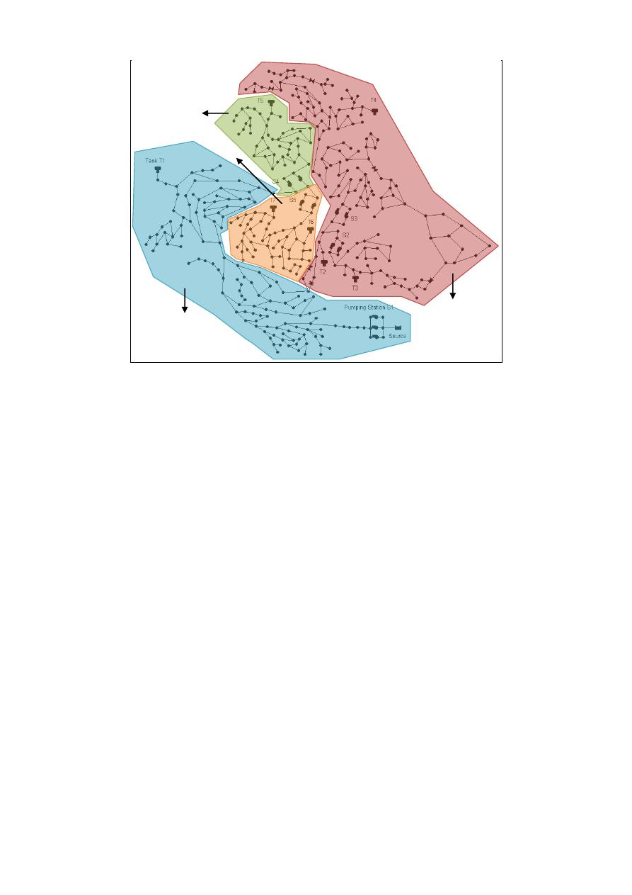
Figure 1: Division of the network according to water supply.
As a result of computing the OPS for the D-Town WDS, a surface considerably different from the
one found when executing the hydraulic simulation in the actual network (for the selected design
scenario) was expected. Hence the objective was to change pipe sizes and eventually pumps trying
to adjust the real surface to the OPS, fulfilling the pressure constraints in an optimal way and
considering as the main objective function, the constructive costs.
In order to adjust the surface, it is necessary to change pipe’s sizes gradually, calculating the
modified surface each time until the pressure constraint is met. Here is where the UP concept is
used to select the order in which the pipes will be modified. The UP of a pipe can be calculated as:
(
)
where UP
p
is the power dissipated by the pipe
, Q
p
is the flow rate on that pipe and h
f
and h
m
are
the friction and minor losses respectively. As the procedure has calculated two pressure surfaces,
there are two UPs for each pipe: the first is the one calculated with the flow and the head difference
between the two nodes that define the pipe, computed with the heads assigned by the OPS, and the
second one is computed with the heads assigned by the real surface. Thus, the difference between
the two UPs is a measure of the difference of the surfaces provided (added) by that particular pipe.
Taking into account that last conjecture and the objective of adjusting the real surface to the OPS,
the UP difference is an acceptable criterion to define the order in which the pipes will be modified
and therefore the OPS and the UP can be used to solve that first D-Town WDSs problem in an
explicit hydraulic-based way. Furthermore, that mentioned methodology allows an easy conjunction
with the solution of the second problem, as it is expected to be solved using that mentioned OPUS
methodology, which is also based on defining an OPS.
The use of OPUS for the second problem requires three executions of the algorithms as the final
topology is not totally defined (the extension of the system can be connected to one of the two
available nodes or both). However this task does not require much computational time as the OPUS
1
2
3
4
methodology is considerably efficient (see Table 1). Therefore the proposed procedure to solve the
second problem is considering that decision variable hence the solution can be quite better than if
assuming a single way to connect the extension.
Once the design is done for the design scenario, an operation optimization is needed. In order to
determine the optimal way, it was extracted the pump series of usage for the modified system. Then
the usage series of each pump were assigned as patterns in the EPANET model. Finally the patterns
are modified to reduce the pumping costs by changing some OPEN status to CLOSED, looking
after each change that the hydraulic conditions are accomplished.
RESULTS
According to Figure 1, the system was divided in four sectors depending on the water supply
characteristics and in this section the results for each one are presented. Taking into account that the
Sector 1 is the upstream sector for the other ones, this was the last one in being analysed. On the
other hand, the Sector 3 was selected to be the first sector to be rehabilitated. With the Sector 3
modified the rehabilitation for the Sector 2 was done and then Sector 4 was modified independently.
Sector 3
The result for the hydraulic execution considering the different scenarios of shut down showed that
even when the tanks were full, some nodes presented critical pressures (under 25.0 m). Based on
that result, it was considered necessary to use diesel generators that allow the pumps to always fulfil
the pressure in these nodes. However the tank T7 with its original size was not enough to ensure
water supply at some hours during the week. In that way it was necessary to increase its size just by
the minimum available volume (500 m
3
). Once this was implemented, the problem could be solved
by changing some of the pipes in the sector.
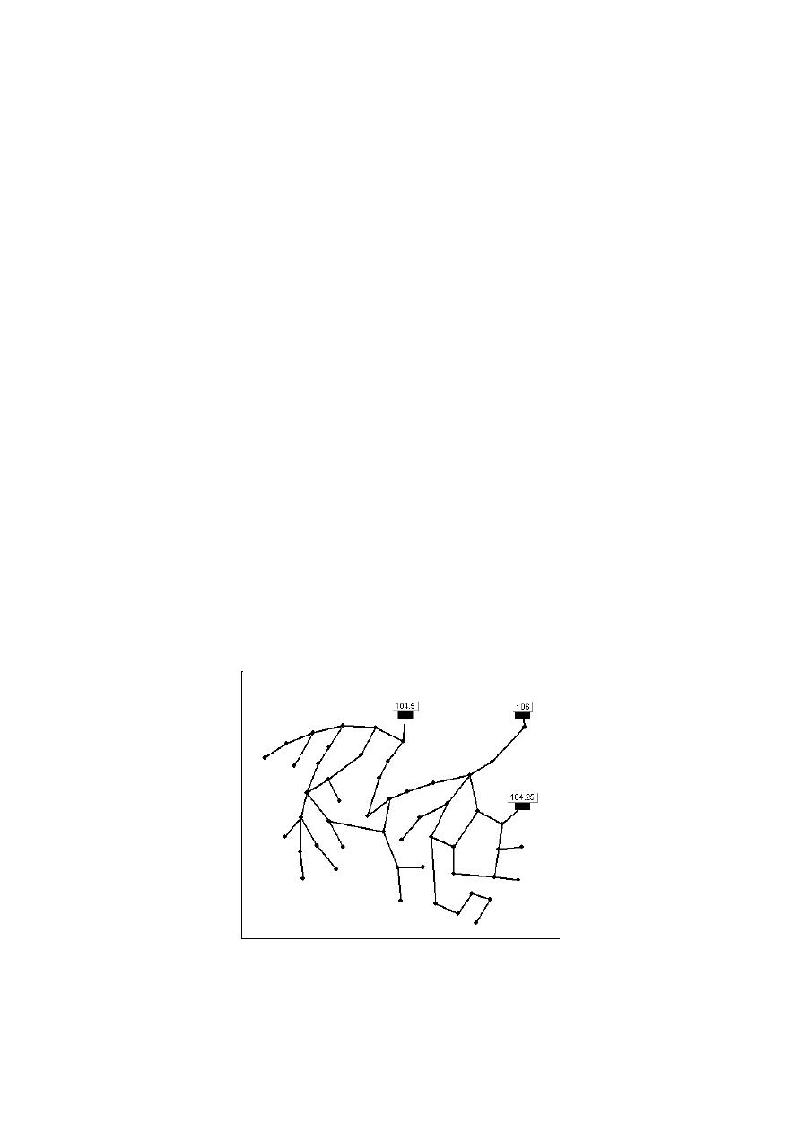
Figure 2 shows the Sector 3 modelled with reservoirs were the total head in the nodes T6 y T7
correspond to the average of the possible heads in the tanks of the original model. For the node J317
the head was near minimum head downstream the pump station on the original model. With this
model a design using OPUS methodology was done in order to calculate the UP difference between
the new design and the actual model.
Figure 2: Sector 3 modelled with reservoirs – Total head in the reservoirs in meters.
According to the methodology, the pipes that had to be changed were the P815 from 102 mm to 203
mm and P752 from 152 mm to 203 mm. An example of the results for the first evaluation of the
difference of UP in the sector is shown in Figure 3, in which can be seen that there is a pipe that
presents a higher value of UP and it corresponds to pipe P815 that was the first pipe changed by the
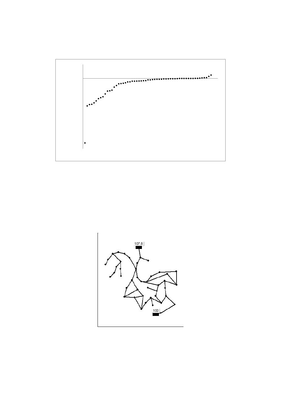
criterion of UP. With the diesel generators, the two increased pipes and the new tank, the hydraulic
conditions were accomplished, when the sector’s upstream node (J302) had at least 2.0 m of
pressure. It meant the resulting usage series of the pumps could be established as patterns in
EPANET for finally change some OPEN status to CLOSED status.
Figure 3: Results of evaluating the difference of UP for Sector 3.
Sector 2
In order to model Sector 2 it was necessary to include in the model the Sector 3 to take into account
the water demand of this one. A reservoir was placed in node J332 with a total head equal to the
minimum required head in this node (61.0 m). After that, the execution that evaluates the system
under shut down scenarios showed that the tank T5 was empty in most of the shut down scenarios.
Taking into account the power required for the average flow in this sector and the cost of the
minimum volume tank, it was decided as cheapest to introduce diesel generators for pump station 4.
Figure 4: Sector 2 modelled with reservoirs – Total head in the reservoirs in meters.
In Figure 4, it is shown the network that allows the OPUS methodology application. After the
difference of UP analysis, it was determined that the only pipe that had to be changed was P853
from 203 mm to 254 mm. Figure 5 shows the ranking of the differences of UP for this sector, and it
can be seen that there is a pipe with a considerably higher difference that corresponds to the pipe
-0.25
-0.20
-0.15
-0.10
-0.05
0.00
0.05
0
10
20
30
40
50
60
Δ
U
P
(
m
4
/s)
Ranking for each pipe
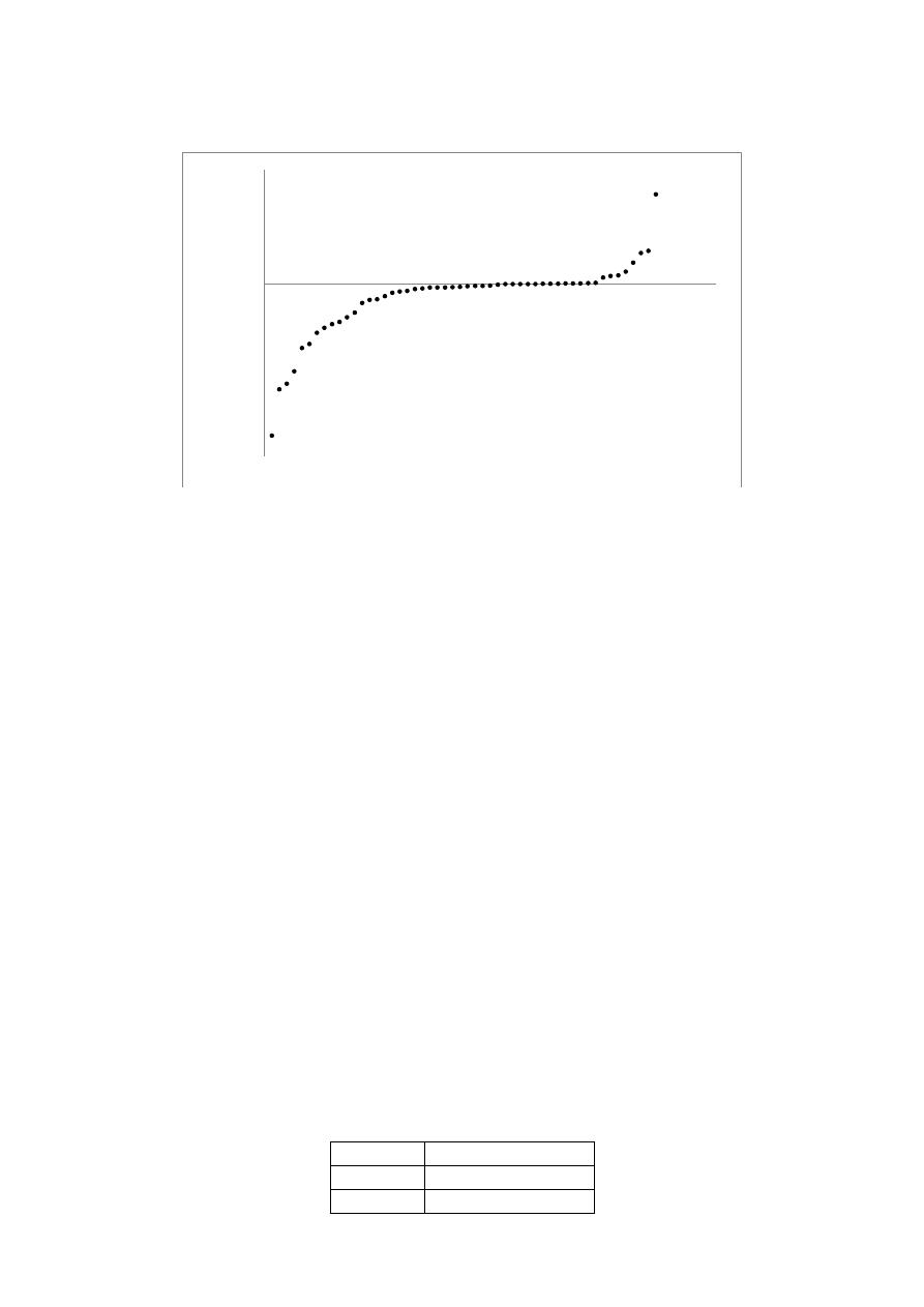
P853. With this actualization of the model, the usage series for PU8 and PU9 were established as
patterns that finally were optimized to reduce operational costs.
Figure5: Results of evaluating the difference of UP for Sector 2.
It is important to mention that after modelling Sectors 2 and 3 connected, it was found that pressure
upstream Sector 3 (node J302) was higher than the one supposed before (2.0 m), so in that way the
pattern for pumps PU10 and PU11 were optimized again.
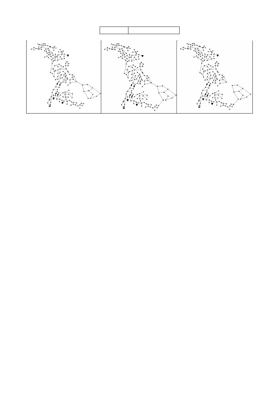
Sector 4
Taking into account that the expansion of the system can be connected to the sector in three
different ways, the current analysis was realized three times for the sector. The first step in each
time, was execute the hydraulics of the system for the different scenarios of shut down and in the
three cases the nodes directly connected to pump station 3 and tank T4 presented deficit of water
supply but the other ones did not. After analysing the pressures in the nodes directly connected to
pump station 2 and tank T3 it was determined that the pumps in station 2 did not required diesel
generators in contrast with pumps of station 3.
In a similar way as with the pump stations, the pipes that were changed in the three cases were the
same according to the results of the UP evaluations. The pipes that were changed were P787 from
102 mm to 152 mm and P1024 from 102 mm to 152 mm. For the design of the expansion, as the
rehabilitation procedure requires a design made by OPUS, the diameter values for those pipes were
instantly calculated during the UP evaluation. For the three cases, the resultant diameters for all the
pipes in the expansion were the minimum one (102 mm).
As before, the usage series for the pumps in station 3 were assigned as patterns that were optimized
to reduce the usage. As the three cases present similar modifications, to define the case to be
implemented an analysis of pump operational costs was done. As shown in Table 2 the case that
presents the most economic pumping costs is case 2. Considering the costs associated with the pipes
in which each case differ for the others, the case 2 remains as the cheapest one.
Table 2: Pumping costs in Sector 4.
Case
Pumping cost ($/yr)
1
112 160
2
104 145
-0.06
-0.05
-0.04
-0.03
-0.02
-0.01
0
0.01
0.02
0.03
0.04
0
10
20
30
40
50
60
Δ
U
P
(
m
4
/s)
Ranking for each pipe
3
108 568
Figure 6: Sector 4– Case 1 (Left), Case 2 (Centre) and Case 3 (Right).
Sector 1
As the Sector 1 is upstream to the three sectors presented before, its rehabilitation was done with a
model of the entire system. The results of executing the hydraulics including the shut down
scenarios showed that tank T1 presented a deficit of water so it required supply from the pumps that
are connected with the reservoir. Additionally to T1, the diesel generators in pump station 1 were
considered as needed to supply water to the other sectors.
Then, the UP was evaluated and after 7 iterations, in which pipe P22 was increased 3 times, from
406 mm to 610 mm, pipe P102 from 508 mm to 610 mm, pipe P100 from 406 mm to 457 mm, pipe
P23 from 508 mm to 610 mm and pipe P995 from 152 mm to 203 mm. The last hydraulic execution
of the UP process showed that the entire system was fulfilling the pressure requirements during the
whole week. Therefore, the optimization of the pumps operation was done for all the pumps on the
system, given the differences in hydraulic behaviour that was observed for the already designed
sectors, when they were connected to Sector 1.
Pumping optimization processes
As a result of the rehabilitation of each sector it was extracted the pump series of usage and
assigned in the EPANET model as it was described in methodology section. The optimization
process of the previous design consisted in changing the pumps status from OPEN to CLOSED at
some hours of the week taking into account that minimum pressures conditions were accomplished
in all demand nodes of the network. In order to optimize the pump series of usage without excessive
computational and human time, changes in these series were made checking the pressure only in
critical nodes of each sector (see Table 4), however when the optimal pattern was reached a
complete inspection was made to verify the operation of D-Town WDS. In addition of minimal
pressure rule it was checked that the final level of all tanks were at least equal or higher than its
initial level.
An optimal pressure time series for node J332 (critical node of sector 1) is shown in Figure 7. It can
be noticed that for the original pump series of usage were several intervals when the pressure was
well above the minimum of 25 m; in these intervals the pump series of usage was modified to
obtain lower pressures. Besides the change of status of the pumps patterns in over pressure intervals
another important criterion was took into account, the hours of the week when electricity tariff was
higher were a priority in the modifications because a pump with an hour in CLOSED status in these
time of the week (27.68 cents/kWh) could represent larger costs savings than an hour in CLOSED
status in another time of the simulation when the electricity tariff was lower (10.94 or 6.72
cents/kWh).
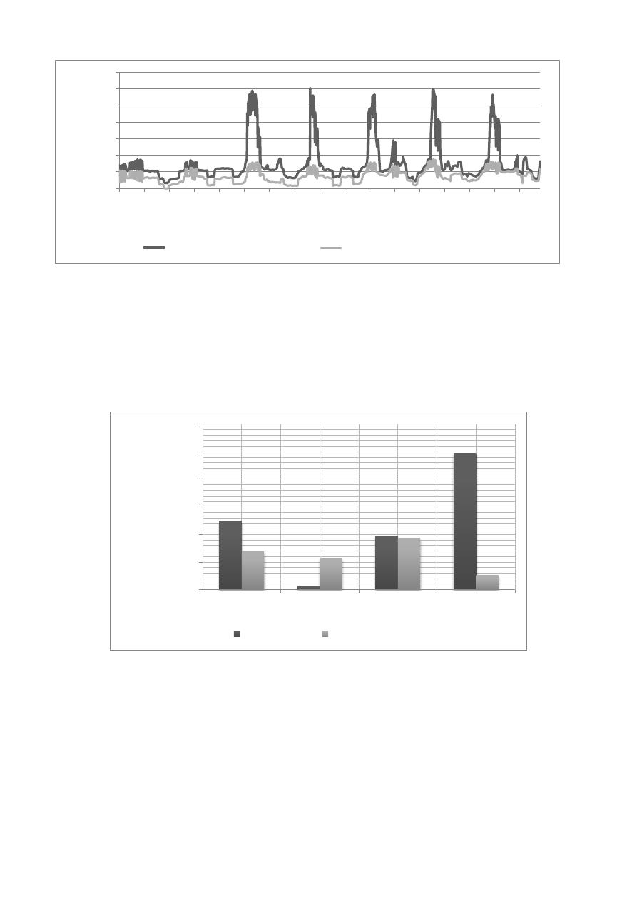
Figure 7: Pressure time series for node J332 – Original and Optimal design.
With these rules all eleven pump series of usage were modified. A comparison between original
patterns costs and optimized ones for Sector 3 is shown in Figure 8. The global pumping cost for
this sector decreased in 48.30%; in the original design were annual pumping costs of $94,759 while
in optimal design were $48,987. It is important to emphasize that at this point, the optimization was
partial because once the entire D-Town WDS was assembled this process was executed again. GHG
emissions also decreased, this time by 47.44%; in first scenario were 1,006,158 kgCO2-e/yr and in
second one were 528,798 kgCO2-e/yr.
Figure 8: Pump annual costs for Sector 3 – Original and Optimized design.
Meanwhile in Figure 9 is shown the same comparison for Sector 1 (entire network). In this figure is
noticed that for most of the pumps the cost is lower in optimized scenario; only for pumps 4, 7 and
9 the second scenario has higher costs. This particular situation is due to the existence of controls in
the EPANET model that turn on these pumps when a tank is near of its minimum level or some
pressure node is close to 25 m. Despite this, global annual pumping costs for entire network were
lower in optimized scenario, before the pumping optimization process the annual cost was $249,992
and after this process was $210,774 for a 16.0% in saving costs. On the other hand, this pumping
optimization process also represents a decrease in greenhouse gas emissions by a 12.0%; in original
scenario it was emitted 2,667,833 kgCO2-e/yr while in optimal design was 2,349,492 kgCO2-e/yr.
25.00
35.00
45.00
55.00
65.00
75.00
85.00
95.00
0
10
20
30
40
50
60
70
80
90
100 110 120 130 140 150 160
P
re
ssu
re
(
m
)
Hour
Original Pump Series of Usage
Optimal Pump Series of Usage
$ -
$ 10,000.0000
$ 20,000.0000
$ 30,000.0000
$ 40,000.0000
$ 50,000.0000
$ 60,000.0000
PU8
PU9
PU10
PU11
A
n
n
u
al
C
os
ts
(U
SD
)
Pump
Original Design
Optimized Design
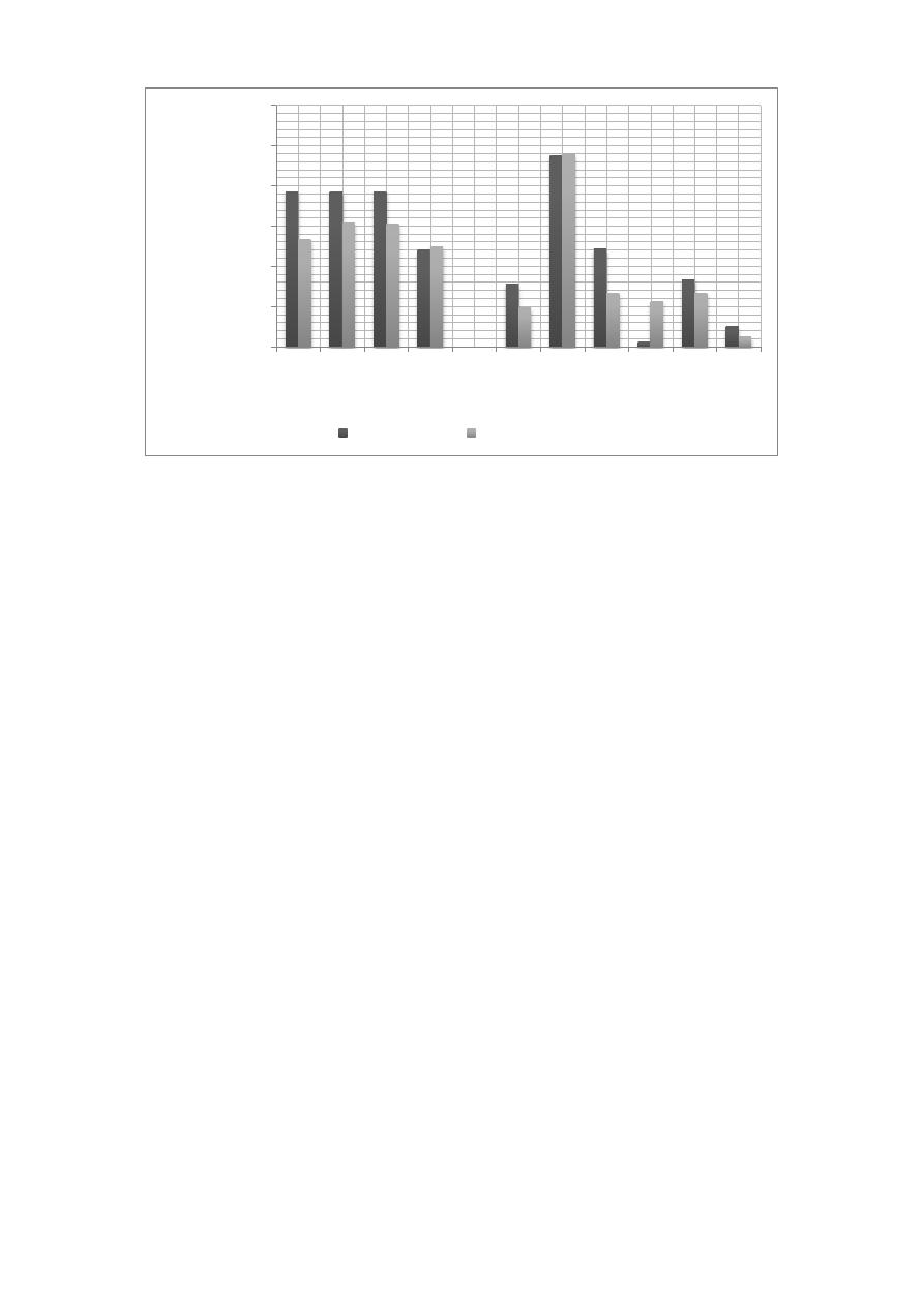
Figure 9: Pump annual costs for Sector 1 – Original and Optimized design.
Final costs
The principal idea of this project is to sort out the actual problem of D-Town in an optimal way.
This means to solve it with the lowest operational and capital cost. Operational costs are related
with the pumps operation or performance; meanwhile the capital costs are associated with any
upgrade done to the existing pumps stations and mainly to the pipe and tank material and
construction.
It is also necessary to reduce de greenhouse gas (GHG) emissions associated with the design, it is
seen as a necessity based in the possibility that in at near future could exist some kind of carbon tax.
In the water case GHG can be subdivided in two parts: capital GHG emissions and operational
GHG emissions. As in the capital costs the capital GHG emission are related to the pipe, tanks and
pumps material and construction, but in this case it is related meanly to the energy required to
produced, transport and install them. In the same way the operational GHG emissions are the result
of the operation of the pumps which get part of their electricity from fuel fossil sources.
Knowing the length and the new diameter of the pipes replaced, the capital GHG emissions is given
by the sum of the product of the length and the annualised EE. As well as in the capital GHG
emissions the capital cost of the pipes, tanks, pumps, diesel generators and valves can be estimated
knowing the length of the pipes replaced, the volume of the new tanks, the model or the curve of
the new pumps, the power of the new diesel generator and the diameter of the valves. The annual
cost of each one of them can be get from the Table 3, 4, 5, 6, 7 included in the PDF which describes
the problem. Then the total capital cost is estimated by the sum of the products of the pipe length
and the annual cost of the new pipe, the sum of the annual cost of the new tanks, new pumps, new
diesel generators and the new valves.
Now, in order to estimate the annual operational costs it’s necessary to compute the weekly cost of
the pump power. The pumps power can be drawn with EPANET which gives information of flows
and the head created by each one, every 15 minutes. The cost of the pump power is the product of
the power and the electricity tariff depending on the hour. Problem description’s Table 8 shows the
energy prices in cents/kWh. In this way the weekly cost pump power is multiplied by the weeks in a
year (52) and then divided in a peak-day factor of 1.3. That’s how the annual operational cost can
be estimated.
$ -
$ 10,000.0
$ 20,000.0
$ 30,000.0
$ 40,000.0
$ 50,000.0
$ 60,000.0
PU1
PU2
PU3
PU4
PU5
PU6
PU7
PU8
PU9 PU10 PU11
A
n
n
u
al
C
os
ts
(U
SD
)
Pump
Original Design
Optimized Design

Similarly to the annual operational cost, the annual operational GHG emissions is the product of the
annual pump energy consumption under normal operation and the emission factor of 1.04 kg-CO2-
e/kWh. The annual pump energy consumption is the sum of the product of the power and the time
(1 hour) during a week, and then this magnitude is multiplied by the weeks in a year (52).
Following the process all ready described the annual capital cost is USD$149,009.01 and the annual
pumping cost is USD$212,791.88. Also the annual capital GHG is 138,371.39 KgCO2-e and the
annual operational GHG is 2,367,847.65 kgCO2-e as shown in Table 3. By his part the water age in
the network is 5.30 hr also shown in the same table.
Table 3: D-Town rehabilitation process results.
Minimizing Costs
Capital Costs
Annual Pipe costs
$92,789.01
$/year
Annual Tank costs
$14,020.00
$/year
Annual Pump costs
-
$/year
Diesel Generator costs
$42,200.00
$/year
Valve cost
-
$/year
Total Annual capital costs
$149,009.01
$/year
Operational cost
Annual Pumping cost
$212,791.88
$/year
TOTAL Annual costs
$361,800.89
$/year
Minimizing GHG emissions
Capital GHG
Annual Pipe GHG
138,371.39
kgCO2-e/year
Operational GHG
Annual Pumping GHG
2,367,847.65
kgCO2-e/year
TOTAL Annual GHG
2,506,219.04
kgCO2-e/year
Minimizing Water Age
WA
net
value (hr)
5.30
DISCUSSION OF RESULTS
To implement this methodology it was necessary an exhaustive analysis process that allows the
understanding of the system. The first step in the understanding of the system consists in perform
different hydraulic executions in EPANET with the objective of analyse the patterns in every
accessory of the system. From this analysis it was possible to establish the way that the all system
was going to be divided in different sectors, each one controlled by pumps stations and tanks that
provide the water required by different nodes.
For the rehabilitation of each sector, it was necessary to implement software in MSExcel with VBA
for Applications joint with the EPANET programmers’ toolkit in order to analyse the behaviour of
each sector when the shut down events occur. The mentioned software facilitates to have an
overview of the pressure and level tanks when the two hours shut down scenario starts in every hour

during the week. The execution time of this software, in a 3.25GB of RAM and Intel Core 2Quad
processor computer, takes about 30 minutes for the shortest sector and 45 minutes for the total
system. Considering that each execution of this software implies 168 shut down events that needs a
computational time lesser than 2.0 seconds to execute a complete week in EPANET, the real time to
run the 168 shut down event corresponds to just 6 minutes being the additional time spent by the
connection between the interface of MSExcel and the Toolkit results.
However the software to model the different sectors in the shut down scenarios needs an important
computational time, this step was just needed four times, each one for each sector. The reason for
this is that, as mentioned in the Results section, the pumps stations in the system required diesel
generators due to tank emptiness and significant low pressures in some nodes. Additionally to the
executions done for each sector, it was necessary to run two more cases that correspond to Sector 4.
The reason for this is that this sector is the only one that has a station without diesel generators. The
absence of diesel generators for this sector implies that, for every pipe that was changed it was
necessary a new execution to check the new hydraulic conditions; so as in Sector 4 there were two
pipe’s change there were needed two executions of the shut down model. It is important to mention
that after the first execution of the shut down model, it was needed a considerably human time to
analyse the results in each sector looking for critical nodes that will the focus nodes for the UP
evaluation. The determined critical nodes for the system are shown in Table 4.
Table 4: Critical nodes for each sector.
Sector
1
2
3
4
Critical node(s)
J332 and J439
J73
J297
J215 and J278
As the OPUS methodology is applied as an comparative design, no discretization process were
performed, implying that the methodology does not require any hydraulic simulation to find the
continuous diameter for each pipe. The computational and human time needed for the UP
evaluation corresponds to determination of UP in each pipe for the two designs available (OPUS
continuous design and original one). Once the pipe that has to be changed was determined, it was
necessary a complete week hydraulic simulation to analyse the time series of the pressure in the
critical nodes. This process of UP evaluation is done whenever a pipe is changed in the sector of
analysis.
In the case of Sector 3, it was necessary to do three UP evaluations; the first one showed that the
first change of diameter was for pipe P815, then a second one was executed before changing pipe
P752 and finally the third one changed again P815. This process stopped when the minimum
pressure during the week was 25.39 m in the node J297 meaning that the pressure requirements
were satisfied for the entire sector.
For Sector 2, it was needed just one UP evaluation in order to satisfy the minimum pressure in the
whole sector. The pipe that was changed after the evaluation was P853 and it leaded to a minimum
pressure in node J73 of 25.06 m.
Sector 4, required two UP evaluations. As it was shown in Table 4, this sector has two critical
nodes. J215 corresponds to the part of this sector supplied by the pump station 2 and tank T3 and
J278 corresponds to the other part of the sector supplied by pump station 3 and tank T4. According
to this subdivision of the sector by the supply characteristics there were done two UP evaluations,
one for each subsector. The results of the evaluations show that, to satisfy the minimum pressure in
J215 the pipe P787 needed to be changed; by the other hand to satisfy the minimum pressure in
J278 pipe P1024 must be changed.
In contrast with the previous sectors, Sector 1 required seven UP evaluations. The reason for this
higher number of UP evaluations is that Sector 1 is the biggest and the demands of this sector
correspond to the accumulated demand for all the system. In Table 5 are the results for each step of
the UP evaluation.
Table 5: UP evaluation in Sector 1.
UP evaluation
1
2
3
4
5
6
7
Pipe to be changed
P22
P22
P102
P22
P100
P23
P995
Initial diameter (mm)
406
457
508
508
406
508
152
Diameter after UP (mm)
457
508
610
610
457
610
203
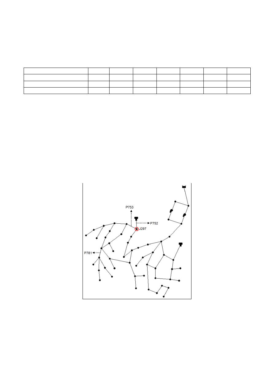
It is important to mention that during the UP evaluation, for each sector, sometimes the pipe with
the highest difference in UP can result in a pipe that does not affect directly the critical node. When
the first pipe in the UP evaluation is not upstream the critical node, the pipe that has to be selected
as the one to be change is the first pipe with the higher difference in the UP and that make part of
the pipes upstream the critical node. For example, in the case of Sector 3, the results of the second
evaluation of UP show that the pipe with the higher difference in UP was P753, but this pipe wasn’t
changed because it is downstream the critical node; similarly the second pipe with higher UP
difference was P781 that is downstream the critical node; Finally the third pipe in the UP ranking
was P752 that is upstream the critical node and affect directly the pressure in that node (see Figure
10).
Figure 10: Sector 3– Pipes found by UP evaluations.
Finally, for the pumping optimization processes were carried out a set number of hydraulic
executions that are shown in Table 6 in order to verify the pressure in nodes and the level of the
tanks. Each hydraulic execution represents an hour of change in the status of some pump usage
series (in the EPANET model an hour change is equivalent to four intervals of 15 minutes).
It is also important to notice that the number of hydraulic executions wasn’t the only way to
determine the computational cost of the pumping optimization process because the time per

execution changed among all the sectors of the network. For example, a hydraulic execution in
sector 3 took roughly a second while an execution in Sector 1 (where the entire network was
included) took 2 seconds. Despite the fact this difference doesn’t seem to matter because both times
are really low the number of executions increase the computational time considerably moreover
because an additional time is required to check the pressure time series of critical nodes as it was
described previously.
Table 6: Hydraulic Executions for Pumping Optimization Processes.
Sector Case Hydraulic Executions
3
-
30
2
-
147
4
1
6
4
2
2
4
3
5
1
-
245
CONCLUSIONS
The main objective of this study was to rehabilitate and design the D-Town WDS. This objective
was accomplished performing a complete analysis of the system and implementing the UP
evaluation methodology with OPUS designs. The actual system is able to supply water to every
node in the original system and its expansion, therefore fulfilling the hydraulic requirements of
minimum pressures.
The UP differences evaluation represents a good methodology to make the changes of pipe
diameters in order to improve the pressures in the system. As shown in this paper by changing a
minimum number of pipes (less than 4.0% of the total number of pipes for the critical sector) it is
possible to achieve more than the minimum pressure in all the nodes.
Due to the efficiency of OPUS methodology to make network continuous designs with a near
optimal cost, the time taken for the rehabilitation of the system results insignificant. In a similar
way the design of the new sector was done with just one hydraulic simulation which required less
than 1.0 seconds.
The possible existence of shut down scenarios controls the way in which the rehabilitation must be
done. With these scenarios the designer can only use diesel generators or increases the volume of
the tanks. Taking into account the pump curves, the flow at the inlet of each sector and the power
generated for each flow, a cost analysis suggested the use of diesel generators in most of the pump
stations during the shut down events.
The optimization process of the pumps usage series patterns represented an improvement in the
operational costs of the pumps stations that resulted in a saving of XX% from the cost before the
optimization.
REFERENCES
Cunham M. and Sousam J. (1999). ““Water distribution network design optimization: Simulated
annealing approach.” Journal of Water Resources Planning and Management. Vol.125
(4):215-221
Eusuff, M. and Lansey, K. (2003“Optimization of water distribution network design using the
shuffled frog leaping algorithm” Journal of Water Resources Planning and Managemen.
129129 (3): 210-225

Geem, Z., (2009). “Particle-swarm harmony search for water network design” Engineering
Optimization, Vol.41 (4): 297-311.
Lin, M., Liu, Y., Liu, G. and Chu, C. (2007). “Scatter search heuristic for least-cost design of water
distribution networks.” Engineering Optimization. Vol. 39 (7): 857-876.
Liong, S. and Atiquzzaman M. (2004). “ Optimal design of water distribution network using
shuffled complex evolution” Journal of the Institution of Engineers. Vol. 44 (1):93-107.
Perelman, L. and Ostfeld, A. (2007). “An adaptive heuristic cross entropy algorithm for optimal
design of water distribution systems.” Engineering Optimization. Vol. 39 (4): 413-428.
Ochoa, S., (2009) “Optimal design of water distribution systems based on the optimal gradient
surface concept” MSc Thesis, Dept. of Civil and Environmental Engineering, Universidad de
los Andes, Bogotá Col. (In Spanish).
Reca, J., Martinez, J., Gil, C. and Baños, R. (2007) “Application of several meta-heuristic
techniques to the optimization of real looped water distribution networks” Water Resources
Management, Vol.22 (10): 1367-1379.
Saldarriaga, J., Takahashi, S., Hernández, F. and Escovar, M. (2011) “Predetermining Pressure
Surfaces in Water Distribution System Design” World Environmental and Water Resources
Congress 2011 ASCE, 93-102.
Saldarriaga, J., Bernal A. and Ochoa, S. (2008) “Optimized Design of Water Distribution Network
Enlargements Using Resilience and Dissipated Power Concepts” Water Distribution System
Analysis 2008 ASCE, 1-15.
Saldarriaga, J., Takahashi, S., Hernández, F. and Ochoa, S. (2010) “An energy methodology for the
design of water distribution systems” World Environmental and Water Resources Congress
2010 ASCE, 4303-4313.
Savic, D. and Walters, G. (1997). “Genetic algorithms for least cost design of water distribution
networks.” Journal of Water Resources Planning and Management, Vol. 123 (2): 67-77.
Villalba, G., (2004) “Combinatory optimization algorithms applied to the design of water
distribution networks” MSc Thesis, Dept. of Systems and Computational Engineering,
Universidad de los Andes, Bogotá Col. (In Spanish).
Wu, I., (1975) “Design of drip irrigation main lines”, Journal of the Irrigation and Drainage
Division , Vol.101 (4):265-278.
Zecchin, A., Simpson, A., Maier, H., Leonard, M., Roberts, A. and Berrisford, M. (2006)
“Application of two ant colony optimisation algorithms to water distribution system
optimization” Mathematical and Computer Modelling Vol.44 (5-6): 451-468.
