
Full Terms & Conditions of access and use can be found at
https://www.tandfonline.com/action/journalInformation?journalCode=nurw20
Urban Water Journal
ISSN: (Print) (Online) Journal homepage: https://www.tandfonline.com/loi/nurw20
Turbulent flow in PVC pipes in water distribution
systems
Juan Carvajal, Willy Zambrano, Nicolás Gómez & Juan Saldarriaga
To cite this article:
Juan Carvajal, Willy Zambrano, Nicolás Gómez & Juan Saldarriaga (2020)
Turbulent flow in PVC pipes in water distribution systems, Urban Water Journal, 17:6, 503-511,
DOI: 10.1080/1573062X.2020.1786137
To link to this article: https://doi.org/10.1080/1573062X.2020.1786137
Published online: 01 Jul 2020.
Submit your article to this journal
Article views: 219
View related articles
View Crossmark data
Citing articles: 1 View citing articles

RESEARCH ARTICLE
Turbulent flow in PVC pipes in water distribution systems
Juan Carvajal, Willy Zambrano, Nicolás Gómez and Juan Saldarriaga
Department of Civil and Environmental Engineering, Universidad de Los Andes, Bogotá, Colombia
ABSTRACT
Since the incorporation of PVC as pipe material in the second half of 20
th
century, its use in the design,
rehabilitation and expansion of Water Distribution Networks (WDS) has been widely assimilated.
However, materials with higher roughness were more commonly used and with these materials were
carried out the studies on which are based the most used design equations (Colebrook-White, Darcy-
Weisbach and Hazen-Williams). In this work, the applicability of these equations is tested using PVC as the
material to verify their precision. Measurements of pressure loss in different assemblies for extents of
Reynolds numbers ranging from 3x10
4
to 5x10
5
and relative roughness between 6x10
-4
and 2x10
-3
were
performed. For small diameters, Blasius and Prandtl–von Kármán equations can be used to calculate the
friction factor. On the other hand, for larger diameters, the Colebrook-White equation correctly describes
the relationship between the friction factor and the Reynolds number.
ARTICLE HISTORY
Received 25 July 2019
Accepted 17 June 2020
KEYWORDS
Head losses in PVC pipes;
steady flow in pressure
conduits; friction factor;
turbulent flow; flow
resistance
Introduction
Water distribution systems (WDSs) are one of the most impor-
tant urban infrastructure assets of the society. They are essen-
tial for human life in cities and directly affect public health.
Therefore, it is vital to understand the hydraulic behavior of
WDSs to properly design and operate them. This work is rele-
vant because it addresses to two basic inquiries: (1) the effect of
modern materials (PVC) in pipes and in the design of civil
infrastructure and (2) if the equations used for calculating the
flow characteristics in pipes are adequate or sufficiently precise.
Testing precision of friction head loss equations is essential
because many researches focus on new methodologies for
more precise designs and do not question if the equations for
the design problem are sufficiently precise.
The rational empirical study of this work is relevant because
the equations used for the design of civil engineering infra-
structure date back to the 19th and early 20th century and
plastic pipes began to be tested, approved and used globally, in
the mid 1960s. Therefore, when the equations were estab-
lished, no tests were performed in this material and it is not
clear if they are precise and should be used for the designs. The
misuses of these equations can translate to capacity problems
in urban drainage systems and distribution of drinking water,
which has serious implications. As mentioned, in a WDS there
can be social, economic and health implications regarding the
errors in the design of these systems. It is likely that, for the
design horizon contemplated, the systems do not fulfill their
function due to blunders in the design calculations.
To have an accurate estimation of the flow resistance within
the system it is necessary to study the equations used for
calculating the flow characteristics in pipes. The most com-
monly used equations for pipe design are Colebrook-White,
Darcy-Weisbach and Hazen-Williams. Although the use of the
Hazen-Williams equation is preferred for its ease of operation,
since it is explicit for velocity, one must be very careful because
it is often overlooked that this equation has limits of applic-
ability (Diskin
1960
). In this research, the equations mentioned
before are used to calculate the friction factor f
ð Þ
in a series of
laboratory tests to verify their validity.
Darcy-Weisbach
Equation (1)
is the most general equation
for determining friction head losses, and thus, it does not have
any limits in its applicability.
h
f
¼
f
l
d
v
2
2g
(1)
where g is the acceleration of gravity, d is the internal diameter
of the pipe, l is the length of the pipe, v is the velocity of the
flow through the pipe and f corresponds to the friction factor.
Colebrook and White (
1939
), on a semi-empirical basis,
found a mathematical relationship to describe the behavior of
the friction factor in the turbulent flow zone:
1
ffiffi
f
p ¼
2log
10
k
s
3:7d
þ
2:51
Re
ffiffi
f
p
�
�
(2)
where f corresponds to the friction factor, Re is the Reynolds
number, d is the internal diameter of the pipe and k
S
=
d
ð
Þ
is the
pipe relative roughness. It is important to denote that f ; Re and
k
s
=
d are all dimensionless parameters. For smooth pipes, if k
s
=
d
= 0,
Equation (2)
can be rewritten into the equation proposed
by Prandtl-von Kármán. This also applies for rough pipes of
uniform roughness, when the value of 1/Re tends to 0
(Finnemore and Franzini
2002
; Quintela
2011
).
The Hazen-Williams
Equation (3)
is shown below:
v ¼ 0:849C
HW
R
0:63
S
0:54
(3)
where v is the velocity, R is the hydraulic radius, S is the energy
loss per length and C
HW
is the Hazen-Williams coefficient. Some
authors have set limits of applicability for this equation:
CONTACT
Juan Saldarriaga
jsaldarr@uniandes.edu.co
URBAN WATER JOURNAL
2020, VOL. 17, NO. 6, 503–511
https://doi.org/10.1080/1573062X.2020.1786137
© 2020 Informa UK Limited, trading as Taylor & Francis Group

Finnemore and Franzini (
2002
) and Houghtalen, Akan, and
Hwang (
2010
) suggest that the equation applies to pipes with
diameters greater than 5 cm and velocities lower than 3 m/s.
Based on contemporary standards for WDSs such as: U.S.
American Water Works Association (AWWA
2002
), Canadian
Design Guidelines for First Nation Water Works (Indian and
Northern Affairs Canada
2006
), Australian Drinking Water
Guidelines (Natural Resource Management Ministerial Council
2011
) and Colombian Technical Regulation of the Drinking
Water and Basic Sanitation Sector (Ministerio de Vivienda,
Ciudad y Territorio
2011
), the investigation focuses in the area
of the Moody diagram in which real designs are contemplated.
In addition, the scope of the research was reduced to PVC pipes
with commercial diameters between 75 mm to 250 mm, which
represent the composition of secondary water distribution net-
works in a community (Ministerio de Vivienda, Ciudad
y Territorio
2011
).
Previous studies
The concern about the difference between modern materials
against those used to study the equations that engineers rely
on to make their designs is not so recent. For smooth pipes, the
experimental determination of roughness k
s
is difficult and is
usually done by statistical analysis. Diogo and Vilela (
2014
),
citing Lencastre (
1996
) and Novais-Barbosa (
1986
), observe
that values of the order of 0.002 mm to 0.004 mm or even
larger are often reported and commonly used in engineering
practice for polyethylene and PVC pipes, and also highlight that
aspects regarding the manufacturing processes or the age of
the materials are not usually considered in the roughness
selection.
Numerous studies have reported that the friction factors
observed and the corresponding head losses in the flow carried
by plastic pipes are usually lower than those obtained when
considering the Colebrook-White equation without absolute
roughness. A succinct and suitable review is presented in
Diogo and Vilela (
2014
) in which it is presented a succinct and
suitable review. Levin (
1972
) presented this for very smooth
plastic pipes of 20 meters long, with an internal diameter of
approximately 210 mm. According to (von Bernuth and Wilson
1989
), Norum (
1984
) and Urbina (
1976
) tested small polyethy-
lene pipes with internal diameters between 8.9 mm and
21 mm, as well as Paraqueima (
1977
), who studied polyethy-
lene pipes with internal diameters of 17.6 mm and 15.5 mm,
respectively. With respect to high Re numbers, Bagarello et al.
(
1995
) carried out tests on small low-density polyethylene
pipes of 100 meters in length and commercial diameters of
16 mm, 20 mm and 25 mm. Cardoso, Frizzone, and Rezende
(
2008
) tested low-density polyethylene pipes with a length of
15 meters and small internal diameters of 12.9 mm, 16.1 mm,
17.4 mm and 19.7 mm.
More recently, Diogo and Vilela (
2014
) conducted a research
in the Laboratory of Hydraulics, Water Resources and
Environment of Coimbra University, Portugal, using three
assemblies with four types of plastic pipes of different dia-
meters: (1) two old PVC pipes with internal diameters of
17.35 mm and 21.75 mm; (2) a high-density polyethylene
(HDPE) pipe with an internal diameter of 53.6 mm; (3) a low-
density polyethylene (LDPE) pipe with an internal diameter of
94.5 mm; and (4) crystal PVC pipe with an internal diameter of
35 mm. The results of the tests showed a trend towards the
Colebrook-White curve that relates the friction factor with the
Reynolds number. Therefore, they confirmed the Colebrook-
White equation as an effective tool for determining continuous
head losses for water flowing through pressure plastic pipes in
turbulent regimes. In addition, for Re up to 1 × 10
5
and a little
less than 1x10
6
, the empirical equations for smooth pipes of
Blasius and Scimemi showed an appropriate behavior. This
article presents an experimental work that is based on the
research work and analysis proposed in Diogo and Vilela
(
2014
). It was performed for PVC pipes of relatively large dia-
meters, such as those that can be normally found in the current
public Water Distribution Networks, and develops, expands and
confirms the previous results obtained by those authors.
Analysis and empirical methods
An inventory of some secondary distribution networks in
Colombian cities was made to confirm the scope of the inves-
tigation. Results obtained showed that pipe diameter distribu-
tion for different secondary networks is analogous and
therefore applicable.
This inventory includes all the materials currently used in
WDS in Colombia (ductile iron, asbestos cement, PVC, PVC-U,
polyethylene and concrete). The showed diameters in the table
correspond to a commercial denomination, they are not the
real internal or external diameters of the pipes.
Table 1
shows similar distributions of pipe diameters for
secondary networks in different cities, all with a tendency to
small diameters up to 150 mm. Additionally, diameters of 50
millimeters exist although the normative does not recommend
them (previous versions of the normative allowed them). Other
secondary networks from different cities also showed alike pipe
distributions.
The Colombian Technical Regulation of the Drinking Water
and Basic Sanitation Sector (RAS
2001
) also establishes recom-
mendations for the different materials that used in a WDS, as
Table 1.
Resume inventory of some secondary distribution networks in Colombian cities. (The represented diameters are commercial and from several materials).
Barrancabermeja
Bogota
(Sector 13)
Bucaramanga (Sector Estadio)
Bogota
(Sector 7)
Santa Marta
(Sector San Jorge)
Diameter (mm)
# of pipes
% of total
# of pipes
% of total
# of pipes
% of total
# of pipes
% of total
# of pipes
% of total
50
837
11%
154
2%
958
14%
24
1%
820
46%
75
4571
61%
2993
41%
4444
64%
1099
29%
536
30%
100
958
13%
1858
25%
828
12%
1172
31%
239
13%
150
482
6%
1539
21%
481
7%
939
25%
79
4%
200
338
5%
528
7%
195
3%
295
8%
64
4%
300
271
4%
317
4%
57
1%
250
7%
34
2%
504
J. CARVAJAL ET AL.
well as the range of velocities to guarantee. For networks using
PVC, minimum velocity: 0.50 m/s and maximum velocity:
6.00 m/s. Likewise, AWWA (
2002
) establishes the following
range for the velocities in PVC: minimum velocity: 0.15 m/s
and maximum velocity: 1.52 m/s.
Using
Equation (4)
and assuming a temperature of 20°C (ν =
1.003 × 10
−6
m
2
/s), is possible to calculate the range of Re that is
permitted in this type of WDS for diameters of 75, 100, 150, 200
and 250 mm. Similarly, the theoretical relative roughness (k
s
=
d)
can be calculated for each diameter knowing that the absolute
roughness (k
s
) of the PVC found in literature is 0.0015 mm. The
results are shown in
Table 2
.
Re ¼
vd
ν
(4)
Larger diameters were not evaluated due to their meager
quantity in percentage founded in secondary networks. In
addition, for larger diameters PVC is not a competitive material.
Pipes with larger diameters are usually made of concrete, GRP
and ductile iron.
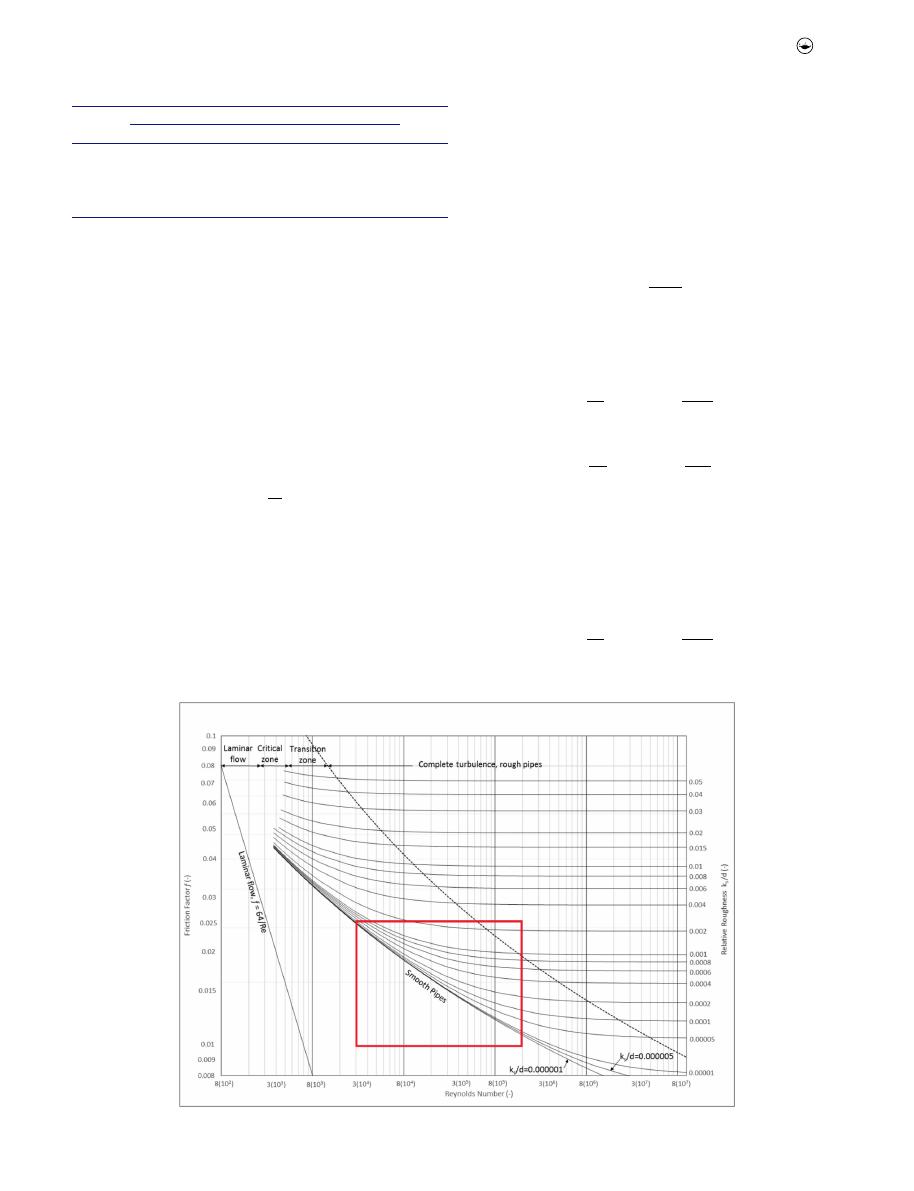
As a result, the area of the Moody diagram of interest when
working with secondary water distribution networks is
enclosed in
Figure 1
.
Often, this is the expected range when working with very
smooth plastic pipes considering the recommendations of
velocities for the design of distribution networks.
To perform an analysis of the data obtained at the time of
the different tests, it is important to delimit the transition zone
in the Moody diagram. For the Hydraulically Smooth Turbulent
Flow (HSTF), the Blasius equation is used to calculate the fric-
tion factor. Blasius (
1912
) found that for Re numbers between
5 × 10
3
and 1x10
5
, the friction factor is calculated with
Equation (5)
.
f ¼
0:316
Re
0:25
(5)
On the other hand, Prandtl (
1925
) found that, for the calculation
of the friction factor for both smooth and rough turbulent flow,
Equations (6)
and (
7
) could be used, respectively.
1
ffiffi
f
p ¼
2log
10
2:51
Re
ffiffi
f
p
�
�
(6)
1
ffiffi
f
p ¼
2log
10
k
s
3:7d
�
�
(7)
According to Colebrook and White (
1939
), a flow may be clas-
sified as HSTF (Hydraulically Smooth Turbulent Flow) when the
pipe roughness size is equal to or less than 30.5% of the
thickness of the viscous laminar sublayer (δ
0
). Then, by repla-
cing the pipe roughness with 0.305δ
0
in the Colebrook-White
equation,
Equation (8)
is obtained.
1
ffiffi
f
p ¼
2log
10
5:21
Re
ffiffi
f
p
�
�
(8)
Table 2.
Reynolds number range and relative roughness, with ks equal to
0.0015 mm, range in secondary WDS.
d (mm)
AWWA
RAS
k
s
/d(-)
Re
max
(-)
Re
min
(-)
Re
max
(-)
Re
min
(-)
75
1:14 � 10
5
1.12 � 10
4
4.49 � 10
5
3.74 � 10
4
0.000020
100
1:52 � 10
5
1.50 � 10
4
5.98 � 10
5
4.99 � 10
4
0.000015
150
2.27 � 10
5
2.24 � 10
4
8.97 � 10
5
7.48 � 10
4
0.000010
200
3.03 � 10
5
2:99 � 10
4
1.20 � 10
6
9.97 � 10
4
0.000008
250
3.79 � 10
5
3.74 � 10
4
1.50 � 10
6
1.25 � 10
5
0.000006
Figure 1.
Area of Moody diagram in which secondary WDS designs are contemplated for PCV pipes.
URBAN WATER JOURNAL
505

This equation establishes the limit between the hydraulically
smooth turbulent flow and the transition turbulent flow in
those cases in which the absolute roughness (k
s
) is not an
absolute value but an equivalent value that represents the
random variability of surface roughness in a normal material.
For that reason, we did not use
Equation 7
because it repre-
sents those cases studied by Johann Nikuradse, which used
a constant artificial roughness created by fixing sand grains
with the uniform diameter with the size is larger than the
laminar sublayer thickness (Streeter, Wylie, and Bedford
1998
).
Therefore, the equations expressing the hydraulically smoot
turbulent flow zone in the Moody diagram are
Equations (5)
, (
6
)
and (
8
).
Equations (5)
and (
6
) are for totally smooth pipes and
they represent a theoretical minimum limit for f; they appear as
the lower limit on Moody Diagram. On the other hand,
Equation (8)
represents the upper limit of hydraulically smooth
turbulent flow as shown in all figures.
The deductive process of
Equation 8
is shown below:
1
ffiffi
f
p ¼
2log
10
0:305δ
0
3:7d
þ
2:51
Re
ffiffi
f
p
�
�
(9)
δ
0
¼
11:6ν
v
�
(10)
(1) Roughness (k
s
) is replaced in
Equation (2)
with 30.5% of
the viscous laminar sublayer (δ ‘)
where ν is the kinematic viscosity of the fluid and v
�
, is the shear
rate velocity that is defined as follows in
Equation (11)
:
v
�
¼
ffiffiffiffi
τ
0
ρ
r
(11)
where τ
0
is the shear stress and ρ the density of the fluid.
(1) In
Equation 9
, the thickness of the viscous laminar sub-
layer is replaced by
Equation (10)
and
Equation (11)
.
1
ffiffi
f
p ¼
2log
10
0:305
3:7d
11:6ν
v
�
þ
2:51
Re
ffiffi
f
p
�
�
1
ffiffi
f
p ¼
2log
10
0:305
3:7d
11:6ν
ffiffiffi
τ
0
ρ
q
þ
2:51
Re
ffiffi
f
p
0
B
@
1
C
A
(12)
f ¼
8τ
0
ρv
2
(13)
(1) The relationship between the friction factor and the
shear stress is considered as shown in
Equation (13)
.
where v is the mean velocity of the flow.
(1) In
Equation (12)
, the shear stress is replaced by the
friction factor, density and average flow velocity
(
Equation (13)
)
1
ffiffi
f
p ¼
2log
10
0:305
3:7d
11:6ν
ffiffiffiffiffi
f ρv2
8
ρ
r
þ
2:51
Re
ffiffi
f
p
0
B
B
@
1
C
C
A
1
ffiffi
f
p ¼
2log
10
2:7ν
ffiffi
f
p
vd
þ
2:51
Re
ffiffi
f
p
�
�
(14)
(1) Finally, in
Equation (14)
the velocity is replaced as
a function of the Reynolds number.
1
ffiffi
f
p ¼
2log
10
2:7ν
ffiffi
f
p
νRe
d
d
þ
2:51
Re
ffiffi
f
p
!
1
ffiffi
f
p ¼
2log
10
2:7
Re
ffiffi
f
p þ
2:51
Re
ffiffi
f
p
�
�
(15)
On the other hand, the upper limit of the transition zone is
defined by the HRTF (Hydraulically Rough Turbulent Flow).
According to Colebrook and White (
1939
), this happens when
k
s
is equal to 6:1δ
0
.
Equation (7)
and
Equation (16)
express the
upper limit of the transition zone.
1
ffiffi
f
p ¼
2log
10
56:6
Re
ffiffi
f
p
�
�
(16)
Equation (16)
is obtained with a deductive similar process to
the one of
Equation (8)
consideringk
s
¼
6:1δ
0
.
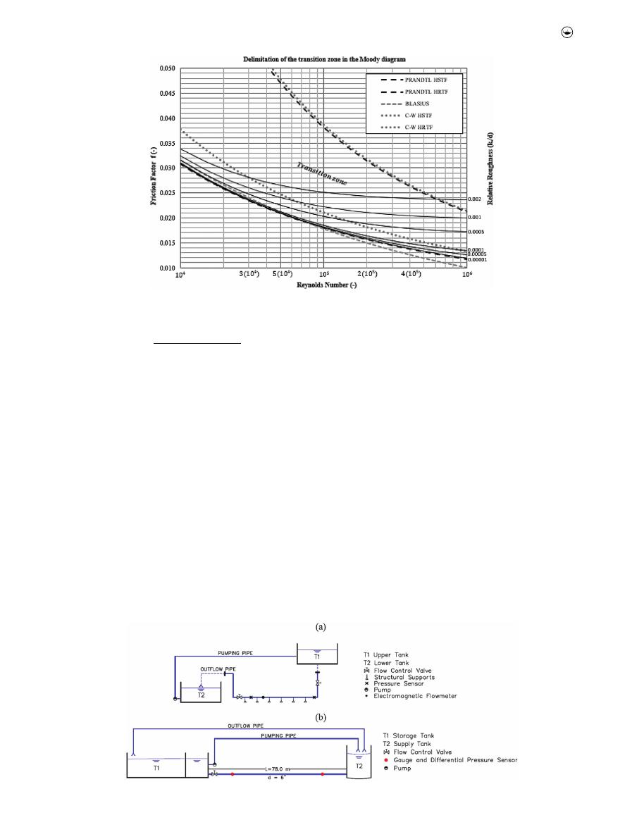
To understand the effect that the new boundaries of the
transition zone can present in the Moody diagram, the lower
and upper limits of the Colebrook-White equation for the tran-
sition zone are plotted based on
Equations (8)
and (
16
). In
addition, the limits of this zone are also defined considering
the Blasius
Equation (5)
and Prandtl-von Kármán
Equations (6)
and (
7
). The delimitation of the transition zone is shown in
Figure 2
, where the x-axis is on a logarithmic scale, the left
y-axis is on a linear scale, and the right y-axis is again on
a logarithmic scale.
When comparing the upper limit of the transition zone
obtained from the Colebrook-White equation with the Prandtl-
von Kármán equation, it is observed that both coincide for all
the range of Re. This occurs because of the second term of the
parenthesis of the Colebrook-White equation is insignificant
compared to the order of magnitude of the first term, as can
be seen in the deductive process of
Equation (16)
. For the lower
limit, the boundary described by the Blasius equation concurs
with what is defined by the Prandtl-von Kármán equation in the
limits of applicability that was deduced. On the other hand, in
contrast to the upper limit, the lower bound defined by the
Colebrook-White
Equation (8)
differs.
Furthermore, in addition to the empirical analysis made for
the equations considering pipe roughness, other widely used
equation to analyze here is the Hazen–Williams equation. The
reason to do so is that this equation is not appropriate for
plastic pipes but, in fact, is commonly and wrongly used. Here
the value of the Hazen-Williams coefficient (C
HW
) must be
determined. A relationship between the C
HW
and f is found
using both the Colebrook-White equation and the Hazen-
Williams equation was given by Liou (
1998
); this relation is:
506
J. CARVAJAL ET AL.
C
HW
¼
14:09
f
0:54
d
0:009
ν
0:081
Re
0:081
(17)
Experiments performed
Seven laboratory tests were performed using two different
experimental installations located in Bogotá, Colombia. Four
tests at the Hydraulic Laboratory of Universidad de Los Andes,
and three tests at PAVCO S.A. facilities (a subsidiary enterprise
of Mexichem, a Mexican producer of plastic pipes and one of
the largest chemicals and petrochemical companies founded in
1953; standard: ASTM D2241) and are schematically repre-
sented in
Figure 3
.
The experimental setup in the Hydraulic Laboratory of
Universidad de los Andes is schematically presented in
Figure
3(a
). The experimental installations consist of an upper tank
(distribution tank to all laboratory location), which serves to
ensure the stability of the pressure head, a lower tank (storage
tank in laboratory underground) and a closed circuit. Water for
the lower tank is pumped to the upper tank (14 m above),
where a constant head is assured to feed the arrangement. To
accomplish this, the pumped discharged to the upper tank
must be larger than the discharged send to the test pipe. The
excess discharge is transported back to the lower tank through
an outflow pipe. The test pipe has 15 mounts that provide
stability and avoid vibrations. The supports are adapted to the
conditions of the laboratory and placed so that the pipe is kept
horizontal. For the differential pressure measurement, there are
two KOBOLD sensors (MAN-SD reference) with a measuring
range of 0–1 bar and an accuracy of ± 0.5%. A portable ultra-
sonic measurer (Ultraflux UF 801-P) is used for measuring velo-
cities. This equipment has a measuring range between 1 mm/s
and 45 m/s, for external diameters between 10 mm and 10
meters, with an accuracy of ± 0.5%. In addition, a Dwyer digital
thermometer (WT-10 model) measures temperature with
a range between −40°C and 200°C and accuracy of ±0.1°C.
Two gate valves regulate the flow that goes through the test
pipe.
The experimental setup in PAVCO facilities,
Figure 3(b
), con-
sists of a test PVC pipe in which the tests are carried out, a pipe
that transports the water from the storage tank to an elevated
Figure 2.
Delimitation of the transition zone in the Moody diagram.
Figure 3.
(a) Schema of experimental setup at Universidad de los Andes. (b) Schema of experimental setup at PAVCO S.A facilities.
URBAN WATER JOURNAL
507

tank (PVC, internal diameter 203.2 mm), and an overflow pipe
(PVC, internal diameter 160.86 mm). There were three test pipes
in molecular bi-oriented PVC as shown in
Table 3
. The supply
tank creates a 6 meters head at the entrance of the test pipe.
This tank is connected to a second pipe that reaches another
tank that fulfills two functions: (1) measures the flow carried
and (2) stores water in the system guaranteeing constant piezo-
metric height to produce permanent steady flow. The flow
measurement is done electronically, using a sharp-crested
weir, and the storage is designed so that the system is fed
continuously by a pumping system, which allows to maintain
a constant redundant flow, avoiding water waste. Additionally,
the system is properly instrumented with electronic measurers
to facilitate pressure and flow measurements, guaranteeing
accuracy and redundancy in them. The instrumentation used
consists in a KOBOLD differential pressure sensor (PAD refer-
ence) and a measurement range of 0–375 mbar with ± 0.075%
accuracy, a flowmeter at the outlet of the test pipe with an
accuracy of ± 0.40%, and a thermometer with an accuracy of ±
0.1°C.
A description of the seven tests performed is shown below:
●
The first test (PAVCO facilities) consisted of a main biaxial
PVC pipe of 78 meters long, with an internal diameter of
161.28 millimeters (without joints).
●
The second test (PAVCO facilities) differs from the first one
as the no-junction (NJ) pipe is replaced with a pipe with
the same diameter but with 13 joints (WJ). The spacing
between joints is 5.85 meters. The type of joint is spigot-
bell and is used to study the influence of fittings on the
hydraulic flow. The instrumentation is maintained the
same as for the first model.
●
The third test, carried out at the Hydraulic Laboratory of
the Universidad de los Andes, consists in a biaxial PVC
pipe of 12 meters in length, without joints (NJ), and a -
161.28 mm of real internal diameter. At the end is located
a gate valve to regulate the flow that goes through the
161.28 mm real diameter pipe. In addition, two grids, with
161.28 mm in diameter and 1 cm thick, were used to
uniformize flow inside the main pipe and ensure uniform
flow conditions.
●
For test 4 (Hydraulic Laboratory), a biaxial PVC pipe is used
with a real diameter of 107.9 millimeters. The length of
this experimental installation is maintained (12 meters),
but spigot-bell joints are used (WJ). The original pipe is
removed and reductions are placed at the beginning and
end of the pipe. The valve is at the end of the pipe, and
the drainage system is the same as mentioned for test 3.
●
In test 5 (Hydraulic Laboratory), a pipe of 107.9 millimeters
of the real diameter without joints (NJ) and 12 meters
long was used. Unlike the other tests, the flow control
valve is located at the beginning of the pipe. At the end of
the assembly, there is located an open tank. For the
determination of the flow, an electronic measuring device
is used.
●
For test 6 (Hydraulic Laboratory), a bonding PVC pipe of
81.84 mm real diameter, with no joints (NJ), and 12 meters
in length is used. The control valve is placed at the end of
the test pipe. For this model, a KOBOLD sensor (PAD
reference) and a measurement range of 0–75 mbar, with
accuracy, up to ±0.075%.
●
For the third PAVCO test (test 7), and last test performed,
the PVC pipe has an internal diameter of 209.42 mm and is
78 meters long. The same amount and distribution of
fittings is maintained as described in the second test
(WJ), as well of the instrumentation used in the first two
tests.
Table 3
provides a summary of the laboratory tests previously
described.
Results, analysis and discussion
For each test, the value of the friction lossesh
f
is measured as
the difference of pressures recorded between the two points
where the piezometers are. In the assemblies that have joints
(spigot-bell), to find h
f
it is necessary to consider the contribu-
tion from minor losses h
m
. These minor losses were calculated
using a loss coefficient of 0.01 (measured in other assemblies of
the Hydraulic Laboratory) per each one of the joints in the
assembly. The minor losses (h
m
) were computed and removed
from the measured total losses (h
f
+ h
m
) in order to obtain the
friction losses (h
f
) and then to calculate the friction factor for all
the cases. It is important to say that in all the tests pipelines
minor losses were up to 0.25% of friction losses in the worst
scenario. Knowing the geometry of the pipe and the flow
velocity that is related to the flow rate recorded in each test,
the friction factor f can be found for each test, as well as the Re
number. With the relation between the friction factor f and the
Hazen-Williams coefficient C
HW
, it is calculated the value of this
coefficient for each test. On the other hand, the k
s
and C
HW
are
calculated from a simple average for all the results performed in
each pipe. A summary of the results is presented in
Table 4
.
The temperature range of water in which the tests were
performed is very stable, no temperature exceeds 23°C and
no one is below 16°C. The range of flow rates has varied
Table 3.
Summary of the laboratory test characteristics.
Laboratory Test
External Diameter
(mm)
Real Internal Diameter
(mm)
Wall Thicknesses
(mm)
Distance between piezometers
(m)
Characteristics
PAVCO S.A (150 – NJ)
168.70
161.28
3.71
66.08
No joints
PAVCO S.A (150 – WJ)
168.70
161.28
3.71
71.24
13 joints
Hydraulic Laboratory (150 – NJ)
168.70
161.28
3.71
11.77
No joints
Hydraulic Laboratory (100 –
WJ)
114.66
107.9
3.38
8.42
2 joints
Hydraulic Laboratory (100 – NJ)
114.66
107.9
3.38
9.51
No joints
Hydraulic Laboratory (75 – NJ)
88.82
81.84
3.49
9.11
No joints
PAVCO S.A (200 – WJ)
219.08
209.42
4.83
73.68
13 joints
508
J. CARVAJAL ET AL.
considerably, and consequently, Re number as well. Test 6 has
the smallest flow value registered, 4.3 liters per second and a Re
number of 6.06 × 10
4
. Test 1 has the largest flow rate, reaching
up to 51 liters per second, Re number of 3.7 × 10
5
. Even with
this considerable flow ranges, changes in temperature, dia-
meter and type of experimental setup, all the data obtained
are in the HSTF regime. Another parameter that is calculated
with the data obtained is the mean Hazen-Williams coefficient
and the mean roughness of the PVC. The mean roughness
presents a great variation when compared to the values regis-
tered in the literature for the PVC (0.0015 mm).
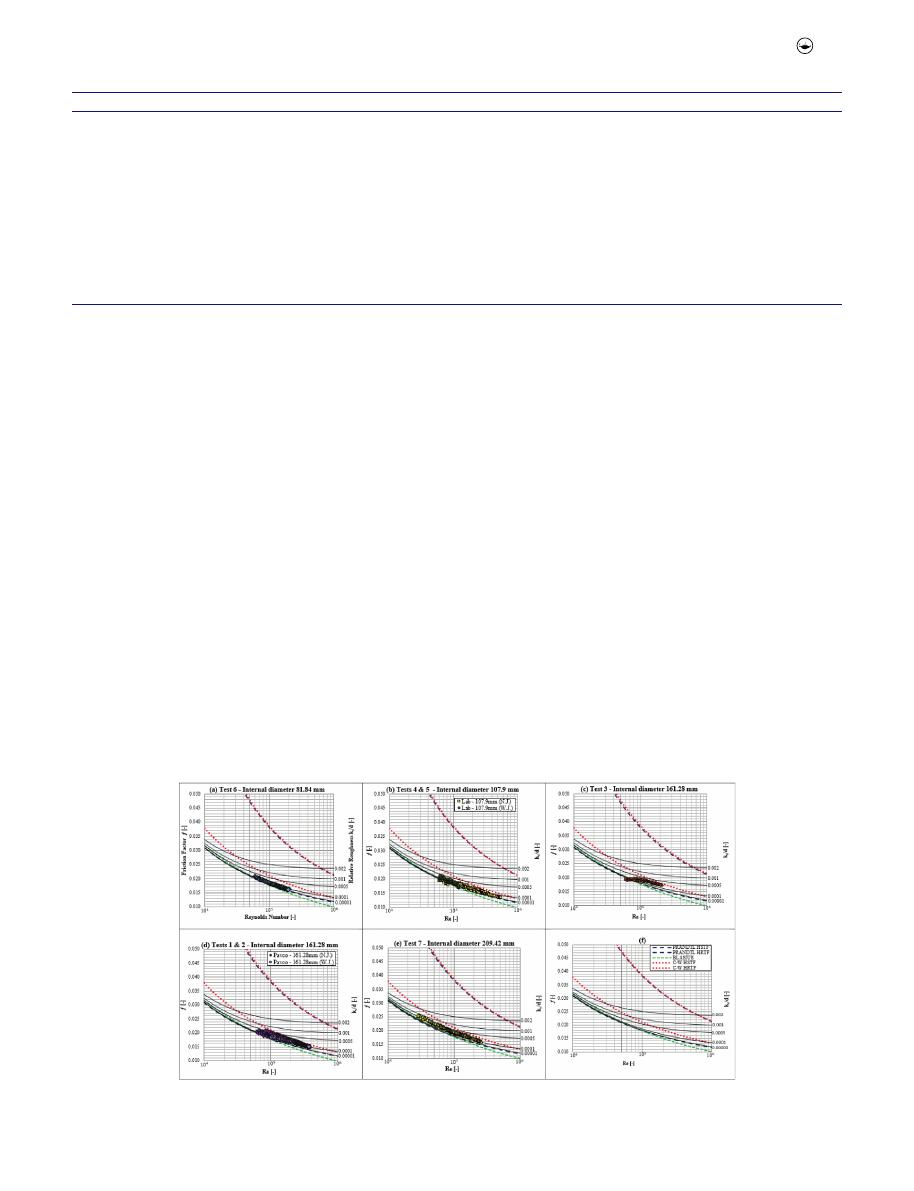
Through
Figure 4(a
–e), the Moody Diagram is shown with
the graphical results of the data obtained for all the tests
performed. The graph results are presented form smallest to
largest diameter.
In
Figure 4(a
), it is shown that for the 81.84 mm real diameter
pipe, the results tend to the limit established by Prandtl von
Kármán for HSTF. For this test, the Re number does not exceed
2 × 10
5
(v ¼ 2.78 m/s).
Figure 4(b
) shows that for Re numbers
between 6 × 10
4
and 1.2 × 10
5
(v ¼ 0.59 m/s – 5.45 m/s), the trend
for a 100 mm commercial diameter PVC pipe (107.9 mm real
internal diameter) is similar with and without joints. Although it
was tested Re numbers up to 5 × 10
5
for pipes without joints, this
region of the Moody diagram cannot be compared since, for pipe
with joints, this range is not covered. However, it is possible to see
that for the entire test range, collected data trend is towards the
boundary of Prandtl von Kármán.
From
Figure 4(c
,d) it is observed that for pipes of 150 mm of
commercial diameter (161.28 mm real internal diameter), the ten-
dency is towards the limit established by the Colebrook-White
equation for HSTF. This trend is clearer when working with high
Re numbers (greater than 1x10
5
; v ¼ 0.7 m/s).
Figure 4(e
) shows
the transition that occurs when working with very low and very
high Re numbers. Towards lower flows, the graph tends towards
the Prandtl von Kármán Smooth Turbulent Flow limit, while for
higher Re number this change, and tends toward the Colebrook-
White Smooth Turbulent Flow limit. For larger diameters, the trend
is most evident toward the Colebrook-White limit.
Figure 5
shows that, in general, for smaller diameters, the
friction factor tends towards the Prandtl von Kármán limit, while
for larger diameters (greater than 161.28 mm in diameter) the
trend tends toward the Colebrook-White limit, for the whole
Table 4.
Summary of results for each test.
Test
T (°C)
Q (l/s)
h
f
(m)
Re (-)
f (-)
k
s
(mm)
C
HW
(-)
1
78 m 150 mm (NJ)
Minimum
16.3
8.24
0.0704
6.26E+04
0.0152
0.0353
146.4
Maximum
20.8
51.02
1.9999
3.70E+05
0.0209
2
78 m 150 mm (WJ)
Minimum
16.4
8.32
0.0677
6.33E+04
0.0148
0.0231
151.0
Maximum
20.2
49.99
2.0992
3.83E+05
0.0199
3
12 m 150 mm (NJ)
Minimum
16.8
9.20
0.0145
6.06E+04
0.0171
0.0334
146.7
Maximum
20.2
33.97
0.1794
2.18E+05
0.0198
4
12 m 100 mm (WJ)
Minimum
20.4
5.58
0.0292
6.05E+04
0.0167
0.0109
149.4
Maximum
22.1
11.35
0.1064
1.24E+05
0.0209
5
12 m 100 mm (NJ)
Minimum
19.9
5.41
0.0305
6.04E+04
0.0135
0.0109
151.1
Maximum
23.0
49.81
1.8012
5.59E+05
0.0210
6
12 m 75 mm (NJ)
Minimum
18.7
4.29
0.0789
6.06E+04
0.0161
0.0075
150.5
Maximum
21.2
14.60
0.7021
2.04E+05
0.0209
7
78 m 200 mm (WJ)
Minimum
16.5
5.11
0.0101
2.86E+04
0.016
0.0706
143.3
Maximum
18.5
45.81
0.5093
2.58E+05
0.0257
Figure 4.
(a) Test 6 – results of 123 tests for PVC pipes with an internal diameter (dÞof 81.84 mm and 66.08 m long (no joints). (b) Test 4 & 5 – results of 145 tests of
l ¼ 9.51 m (no joints) and 132 tests l ¼ 8.42 m (with joints) for d ¼ 107.9 mm. (c) Test 3 – results of 198 tests d ¼ 161.28 mm and l ¼ 11.77 m (no joints). (d) Test 1 &
2 – results of 250 tests of l ¼ 66.08 m (no joints) and 296 tests of l ¼ 71.24 m (with joints) for d ¼ 161.28 mm. (e) Test 7 – results of 186 tests d ¼ 209.4 mm and
l ¼ 73.68 m (with joints). (f) Moody Diagram with the limits established by the proposed equations of different authors.
URBAN WATER JOURNAL
509
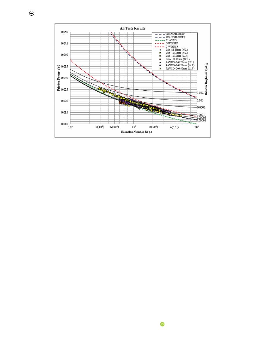
range of Re number in which the data were collected. In addition, it
is clear that for low Re numbers, there is no clear trend. The
dispersion in this zone may be due to the underestimation of the
pressure loss read by the sensors. This variation in the pressure
difference may also lead to an underestimation of the friction
factor and, hence, of relative roughness.
Conclusions
It is normal to question the materials implemented in finding
the design equations most used for the design of potable water
distribution networks. More modern and smoother materials
are being used every day, with the incorporation of thermo-
plastic materials and smoother composite materials. In this
research, the existence of HSTF in PVC pipes that are in the
design range for secondary drinking water distribution net-
works is verified based on the limits established by the pro-
posed equations of different authors.
For a Reynolds number range between 5 × 10
4
and 5x10
5
, it
can be concluded that: for small diameters, the Prandtl von
Kármán equation (
Equation 6
) has an adequate behavior because
allows a good approximation when relating the friction factor (f)
with the Reynolds number (Re), while for larger diameters this
relationship is best described by the Colebrook-White Equation.
This conclusion is relevant because the Prandtl von Kármán HSTF
equation does not use the pipe roughness for the calculation of
the friction factor; hence, it could be irrelevant the estimation of
pipe absolute roughness for the design. Regarding the presence
of joints, it is important to say that they were not a factor that
greatly affected friction head loss in all tested PVC pipes.
For the discharges range used in this research, Hazen-
Williams coefficients show a large variation of about ±12% for
a mean value. This precision is even less for Reynolds numbers
outside of those used in this research, this allows us to conclude
that Hazen-Williams equation should not be used in plastic
pipes.
Even though the materials used for this study are smoother
than the ones to postulate the equations that are currently
used for the estimation of the friction factor, the results show
that traditional equations allow a good approximation to cal-
culate the friction factor. This can be seen in the information
shown, since all the experimental data is located between the
Prandtl von Kármán and Colebrook-White limits, confirming
that the last one, is the most powerful tool for determining
head loses.
With the advancement in new materials and more
powerful tools for data collection, it is essential that new
tests be carried out to corroborate the results attained. By
obtaining even more accurate data, it will be possible to
carry out a more detailed and precise analysis of the
information, thus recreating conditions for a better under-
standing of the reality that occurs in potable water dis-
tribution networks. It is recommended that new tests be
performed, and other modern materials are tested, obtain-
ing even more significant results capable of reaffirming
that the equations that have been used since the
1920s for the design of WDNs are correct and precise.
Disclosure statement
No potential conflict of interest was reported by the author(s).
ORCID
Juan Saldarriaga
http://orcid.org/0000-0003-1265-2949
Figure 5.
All tests results.
510
J. CARVAJAL ET AL.

References
AWWA (American Water Works Association).
2002
. PVC Pipe-Design and
Installation. 2nd ed. Denver.
Bagarello, V., V. Ferro, G. Provenzano, and D. Pumo.
1995
. “Experimental
Study on Flow-Resistance Law for Small-Diameter Plastic Pipes.” Journal
of Irrigation and Drainage Engineering 121 (5): 313–316. doi:
10.1061/
(ASCE)0733-9437(1995)121:5(313)
.
Blasius, H.
1912
. “Das Aehnlichkeitsgesetz bei Reibungsvorgängen in
Flüssigkeiten.” Mitteilungen über Forschungsarbeiten auf dem Gebiete
des Ingenieurwesens, vol. 134. Berlin: VDI-Verlag. doi:
10.1007/978-3-662-
02239-9
Cardoso, G., J. A. Frizzone, and R. Rezende.
2008
. “Fator de Atrito Em Tubos
de Polietileno de Pequenos Diámetros.” Acta Scientiarum – Agronomy 30
(3): 299–305.
Colebrook, C. F. and C. M. White.
1939
. “Turbulent Flow in Pipes, with
Particular Reference to the Transistion Region between the Smooth
and Rough Pipe Laws.” Journal of the Institution of Civil Engineers 11
(4): 133–56. doi:
10.1680/ijoti.1939.13150
.
Diogo, A. F., and F. A. Vilela.
2014
. “Head Losses and Friction Factors of
Steady Turbulent Flows in Plastic Pipes.” Urban Water Journal 11 (5):
414–425. doi:
10.1080/1573062X.2013.768682
.
Diskin, M. H.
1960
. “The Limits of Applicability of the Hazen-Williams
Formula.” La Houille Blanche 6 (6): 720–726. doi:
10.1051/lhb/1960059
.
Finnemore, E. J., and J. B. Franzini.
2002
. Fluid Mechanics with Engineering
Applications. 10th ed. Boston, Massachusetts: McGraw-Hill.
Houghtalen, R. J., A. O. Akan, and N. H. C. Hwang.
2010
. Fundamentals of
Hydraulic Engineering Systems. Englewood, New Jersey: Prentice Hall.
Indian and Northern Affairs Canada.
2006
. Design Guidelines for First Nations
Water Works. Gatineau, Quebec.
https://www.aadnc-aandc.gc.ca/eng/
1100100034922/1100100034924
Lencastre, A.
1996
. Hidráulica Geral. Edição Do Autor. Lisboa, Portugal:
Armando Lencastre.
Levin, L.
1972
. “Étude Hydraulique de Huit Revêtements Mintérieurs de
Conduites Forcées.” La Houille Blanche, no. 4: 263–278. doi:
10.1051/
lhb/1972020
.
Liou, C. P.
1998
. “Limitations and Proper Use of the Hazen-Williams
Equation.” Journal of Hydraulic Engineering 124 (9): 951–954.
doi:
10.1061/(ASCE)0733-9429(1998)124:9(951)
.
Ministerio de Vivienda, Ciudad y Territorio.
2011
. Reglamento técnico del
Sector de Agua Potable y Saneamiento Básico - RAS: TÍTULO B. (2). Bogotá
DC, Colombia: Viceministerio de Agua y Saneamiento Basico. ISBN:
978–958–8491–51–6.
Natural Resource Management Ministerial Council.
2011
. Australian
Drinking Water Guidelines 6. Canberra.
www.nhmrc.gov.au
Norum, E. M.
1984
. “Determining Friction Loss in Polyethylene Pipe Used for
Drip Irrigation Laterals.” Irrigation Age 26: 17–18.
Novais-Barbosa, J.
1986
. Mecânica dos Fluidos e Hidráulica Geral. Vol. 2 vols.
Porto, Portugal: Porto Editora. ISBN: 9789720060211.
Paraqueima, J. R.
1977
. “Study of Some Frictional Characteristics of Small
Diameter Tubing for Trickle Irrigation Laterals.” Thesis (MSc),
Department of Agricultural and Irrigation Engineering, Utah State
University.
Prandtl, L.
1925
. “Uber die Ausgebildete Turbulenz.” Zamm 5 (2): 136–139.
doi:
10.1002/zamm.19250050212
.
Quintela, A. D. C.
2011
. Hidráulica. 10th ed. Fundação Calouste Gulbenkian.
Lisboa, Portugal: Serviço de Educação e Bolsas.
RAS.
2001
. “Reglamento técnico del Sector de Agua Potable y Saneamiento
Básico - RAS: TÍTULO B. (2)”. Bogotá DC, Colombia: Ministerio de
Vivienda, Ciudad y Territorio. Viceministerio de Agua y Saneamiento
Basico. Retrieved from ISBN: 978-958-8491-51-6.
Saldarriaga, J. 2019. Hidráulica de Tuberías. 4th ed. Bogotá: Alfaomega
Colombiana. ISBN:978–958–778–624–8.
Streeter, V. L., B. E. Wylie, and K. W. Bedford.
1998
. Fluid Mechanics. 9th ed.
New York: McGraw-Hill. ISBN: 0–07–062537–9.
Urbina, J. L.
1976
. “Head Loss Characteristics of Trickle Irrigation Hose with
Emitters.” Thesis (MSc), Department of Agricultural and Irrigation
Engineering, Utah State University.
von Bernuth, R. D., and T. Wilson.
1989
. “Friction Factors for Small Diameter
Plastic Pipes.” Journal of Hydraulic Engineering 115 (2): 183–192.
doi:
10.1061/(ASCE)0733-9429(1989)115:2(183)
.
URBAN WATER JOURNAL
511
