
water
Article
Sewer Network Layout Selection and Hydraulic
Design Using a Mathematical
Optimization Framework
Natalia Duque
1,2,3
, Daniel Duque
4,5
, Andrés Aguilar
3
and Juan Saldarriaga
6,
*
1
Eawag, Swiss Federal Institute of Aquatic Science and Technology, 8600 Dübendorf, Switzerland;
natalia.duquevillarreal@eawag.ch
2
Institute of Environmental Engineering, ETH Zurich, 8093 Zurich, Switzerland
3
Water Distribution and Sewerage Systems Research Center, University of the Andes,
111711 Bogotá, Colombia; af.aguilar691@uniandes.edu.co
4
Department of Industrial Engineering, Center for the Optimization and Applied Probability,
Universidad de los Andes, 111711 Bogotá, Colombia; d.duque25@gmail.com
5
Department of Industrial Engineering and Management Sciences, Northwestern University, Evanston,
IL 60208, USA
6
Department of Civil and Environmental Engineering, Water Distribution and Sewerage Systems Research
Center, University of the Andes, 111711 Bogotá, Colombia
*
Correspondence: jsaldarr@uniandes.edu.co
Received: 13 October 2020; Accepted: 20 November 2020; Published: 27 November 2020
Abstract:
This paper proposes an iterative mathematical optimization framework to solve the layout
and hydraulic design problems of sewer networks. The layout selection model determines the
flow rate and direction per pipe using mixed-integer programming, which results in a tree-like
structured network. This network layout parametrizes a second model that determines hydraulic
features including the diameter and the upstream and downstream invert elevations of pipes using
a shortest path algorithm. These models are embedded in an iterative scheme that refines a cost
function approximation for the first model upon learning the actual design cost from the second
model. The framework was successfully tested on two sewer network benchmarks from the literature
and a real sewer network located in Bogotá, Colombia, that is proposed as a new instance. For both
benchmarks, the proposed methodology found a better solution with up to 42% cost reduction
compared to the best methodologies reported in the literature. These are near-optimal solutions
with respect to construction cost that satisfy all hydraulic and pipe connectivity constraints of a
sewer system.
Keywords:
sewer network design; layout selection; hydraulic design; mix-integer programming;
dynamic programming
1. Introduction
A sewer network is an infrastructure that fundamentally comprises pipes and manholes, and is
characterized by a network layout and a hydraulic design. The layout of a sewer network defines the
flow direction within the network following a tree-like structure where all manholes are connected to
the outfall through a unique path. Given a layout, a hydraulic design establishes the diameter for each
pipe and the invert elevation of its two endpoints. The sewer network design (SND) problem aims to
obtain a minimum-cost design capable of transporting a specific flow rate for each pipe, while satisfying
all hydraulic and operational constraints to comply with local regulations. The input information for
Water 2020, 12, 3337; doi:10.3390
/w12123337
www.mdpi.com
/journal/water

Water 2020, 12, 3337
2 of 22
the SND problem includes inflows at each manhole (rain and
/or wastewater), topographic information,
available pipe materials and diameters, density and water viscosity, and hydraulic design constraints.
Significant literature addresses the SND problem. The predominant approach to solve the problem
considers the layout selection (LS) and hydraulic design (HD) as independent (and subsequent)
problems. This separation allows for tractability of the problem at the price of design optimality.
In what follows, we summarize some of the heuristic and exact techniques that have been proposed in
literature to address the LS and HD problems.
A group of studies solve the HD problem for a given layout using mathematical programming
(MP) approaches, such as linear programming (LP) [
1
–
4
]; non-linear programming (NLP) [
5
,
6
];
and dynamic programming (DP) [
7
–
9
]. A DP approach su
ffers from the problem of dimensionality
in its application in the design of sewer systems [
10
]. To improve the dimensionality of DP-like
approaches, Duque et al. [
9
] propose a graph modelling framework for the design of a series of pipes.
The arcs of a graph model di
fferent combinations of invert elevations and diameters, a path represents
a feasible hydraulic design and the best hydraulic design is obtained by means of a shortest path (SP)
algorithm. Since these MP-based approaches can be computationally expensive, some authors use
metaheuristics that provide a good solution with less computational resources. Genetic algorithms
(GA) have been applied to water and sewer engineering problems to obtain least-cost designs [
11
–
13
].
Due to the high adaptability of GAs, they have also been used in combination with other models for
sewer networks design. Cozzolino et al. [
14
] propose a combination with hydrologic and hydraulic
models, Cisty [
15
] couples a GA with LP, Haghighi and Bakhshipour [
12
] with integer programming,
and Hassan et al. [
16
] with heuristic programming (HP). Other heuristic approaches used to solve
the hydraulic design problem are ant colony optimization (ACO) [
17
,
18
], simulated annealing (SA)
together with tabu search (TS) [
19
,
20
], particle swarm optimization (PSO) [
21
], and cellular automata
(CA) [
22
,
23
]. Zaheri et al. [
24
] implemented a two-phase simulation-optimization method to define
iteratively the HD with CA while EPA SWMM is used to simulate the network. These heuristic
strategies do not have optimality guarantees, and the burden to achieve globally optimal designs might
be further expanded since the problem is solved sequentially.
Some authors have addressed the LS problem independently from the HD. This sub-problem is
considered a hard problem that grows exponentially with the number of pipes. Walters [
8
] uses DP for
optimizing the layout of a sewer network by selecting the position of all manholes along the trunk
sewer after determining the order in which branches connect into it. Navin et al. [
25
] use Kruskal’s
algorithm to find the minimum spanning tree (MST) over a base graph in which edge lengths serve as
the weights. From the MST, the authors generate a predefined number of trial spanning trees for the
HD problem. Hsie et al. [
26
] propose a Steiner minimal tree (SMT) problem solved with a mixed-integer
programming (MIP) to select a layout. The objective function minimizes the buried depth of the pipes
assuming that they represent the main construction costs in sewer systems. The construction cost
for the pipes is simplified as a constant cost per unit length, which considers pipe and excavation
costs. Moreover, the methodology uses fixed design parameters (e.g., Manning’s roughness coe
fficient,
filling ratio and minimum and maximum velocities) for the formulation of linear equations in the
MIP. Some metaheuristics have also been used to solve the LS, such as GA [
27
,
28
] and ACO [
29
].
Haghighi [
28
] develops a loop-by-loop cutting algorithm in which he applied GAs for determining the
near-optimal layout using graph theory. The loop-by-loop cutting algorithm has been successfully
used to select those pipes of a base network that can be ‘cut’ to generate an open network layout.
Later, Haghighi and Bakhshipour [
20
] use TS coupled with the loop-by-loop cutting algorithm for
the optimization of the LS and HD. Other studies optimize both the layout and hydraulic design,
yet in a sequential fashion. Moeini and Afshar [
18
,
30
] use a tree-growing algorithm (TGA) to generate
layouts, ACO to determine pipe diameters and NLP to determine pipe slopes [
31
]. Navin et al. [
32
]
use a combination of an MST for the layout selection and modified particle swarm optimization for the
hydraulic design. Other approaches that sequentially solve both problems include [
33
–
37
]. In particular,
Li and Matthew [
34
] are among the first authors to tackle both problems. Their method uses an SP

Water 2020, 12, 3337
3 of 22
spanning tree to obtain a first layout, diameters are derived from hydraulic principles, and invert
elevations are computed using discrete di
fferential dynamic programming (DDDP). The layout is
iteratively improved using the search direction method that identifies pipes for which the flow rate can
be adjusted to decrease the costs, while keeping the remaining pipe weights constant.
In this paper we propose an iterative method to solve the SND problem in which the network
layout and the hydraulic design are computed with exact methodologies. Our method relies on
MIP to obtain a network layout and uses DP to obtain a hydraulic design. The latter is an extension
of the methodology proposed by Duque et al. [
9
] originally intended for series of pipes in sewer
systems. An important feature of our methodology is that the mathematical model that describes each
problem approximates the cost of a complete design using di
fferent but aligned objective functions.
The objective function in the hydraulic design is a better representation of the real cost of a system
because it is based on the diameters and invert elevations of the pipes, which are unknown in the
LS problem. To circumvent this problem, our iterative scheme arises as a mechanism to refine an
approximation of the objective function in the model for the LS problem by regressing previous layout
decisions with their corresponding cost of the optimal hydraulic design. Refining the cost function
approximation improves network layout in terms of the overall design cost, significantly reducing the
optimality burden that arises from decoupling the problems.
Our methodology is novel with respect to previous literature in several aspects. For starters,
any procedure for the layout selection relies on a surrogate for the cost function. For example,
Navin et al. [
25
] use pipe lengths as a surrogate for the cost when computing the MST,
while Hsie et al. [
26
] use ground cutting cost (expressed as a linear function of the invert elevations)
plus a constant value that resembles the pipe cost per unit length. Our surrogate for the cost function
approximates the construction cost of each pipe as a linear function of the flow direction and the
flow rate, and the parameters of such functions are updated at every iteration. The simplicity of
the cost function allows for a tractable model while the function updates help to guide the global
search towards a near-optimal layout. Moreover, when solving the hydraulic design for a specific
layout, there is a choice between solving for diameters and slopes sequentially or jointly. For example,
Li and Matthew [
34
] fix pipe diameters based on design principles and solve a DP to define the crown
elevations at the extremes of the pipes. Moeini and Afshar [
18
,
30
] use ACO to select diameters for
each pipe and derive slopes assuming a maximum flow depth and a fixed elevation at the root node.
Moeini and Afshar [
31
] extend the procedure in [
18
] and derive slopes by heuristically solving an NLP
via BFGS algorithm (see e.g., Nocedal and Wright [
38
] for BFGS optimality conditions). In contrast,
our methodology jointly optimizes both diameter and invert elevations with an exact method, i.e.,
for a fixed layout our hydraulic design is optimal. Lastly, we argue that our iterative scheme is unique
across all methods discussed so far. Most heuristics rely on randomized procedures [
18
,
30
,
31
] or layout
enumeration [
25
,
32
] to obtain di
fferent designs across iterations. Few authors incorporate a tabu list to
guide the global search [
30
,
31
]. A notable exception is Li and Matthew [
34
] with their search direction
algorithm, which essentially leverages the gradient of the objective function to update the current
layout. Our approach is fundamentally di
fferent and proves effective to addressing the sewer design
problem. To summarize our contributions:
•
we propose an MIP to model the LS problem over a network with general topography,
•
we extend the methodology in Duque et al. [
9
] to generate a hydraulic design, and
•
we propose a novel iterative scheme in which the objective function in the LS model approximates
the true hydraulic-based cost, and this approximation is refined as the method progresses.
Hereafter, the paper is organized as follows: the next section provides a rigorous description
of the problem statement and defines key concepts that we use throughout the development of our
methodology, and the subsequent section describes the proposed methodology in detail. Afterwards,
two benchmark instances from the literature and one case study in Bogotá (Colombia) illustrate the
Water 2020, 12, 3337
4 of 22
performance of the methodology. Finally, the last section concludes the paper and outlines future
research avenues.
2. Problem Statement and Definitions
In this section, we provide a formal problem statement of the LS and the HD, as well as the general
design assumptions and terminology used in our methodology. Both problems are modelled using
graph theory [
39
]. Each problem uses a particular graph representing di
fferent features of the network.
The LS graph is connected to the HD graph through an auxiliary graph, the tree-structured graph,
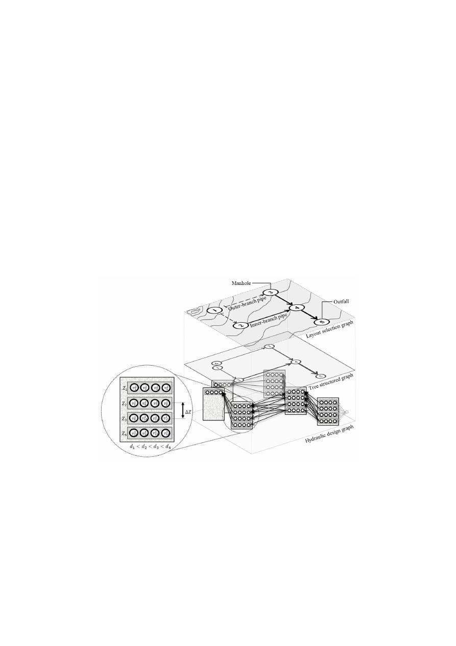
which translates the layout graph into an open network (Figure
1
). The layout selection graph (top)
represents the network topology and is based on manholes, pipes and an outfall. The tree-structured
graph (middle) is the representation of the layout as a tree-like open network by using additional
nodes to represent all the manholes at the extremes of the branches. Later, the hydraulic design
graph (bottom) is built following the tree-structured graph’s connectivity and generates a set of design
nodes for each tree-node in the middle graph, which at the same time belongs to a manhole on the
top graph. Design nodes are used to establish the position and dimensions of the pipes. Therefore,
there are as many design nodes for one manhole as combinations of available pipe diameters and
invert elevations. Possible invert elevations start at the minimum excavation limit and decrease based
on a fixed elevation change (
∆Z), until the maximum excavation limit. The relationship between the
graphs will be explained along with the mathematical formulation of the optimization framework.
Water 2020, 12, x FOR PEER REVIEW
4 of 22
2. Problem Statement and Definitions
In this section, we provide a formal problem statement of the LS and the HD, as well as the
general design assumptions and terminology used in our methodology. Both problems are modelled
using graph theory [39]. Each problem uses a particular graph representing different features of the
network. The LS graph is connected to the HD graph through an auxiliary graph, the tree-structured
graph, which translates the layout graph into an open network (Figure 1). The layout selection graph
(top) represents the network topology and is based on manholes, pipes and an outfall. The tree-
structured graph (middle) is the representation of the layout as a tree-like open network by using
additional nodes to represent all the manholes at the extremes of the branches. Later, the hydraulic
design graph (bottom) is built following the tree-structured graph’s connectivity and generates a set
of design nodes for each tree-node in the middle graph, which at the same time belongs to a manhole
on the top graph. Design nodes are used to establish the position and dimensions of the pipes.
Therefore, there are as many design nodes for one manhole as combinations of available pipe
diameters and invert elevations. Possible invert elevations start at the minimum excavation limit and
decrease based on a fixed elevation change (∆Z), until the maximum excavation limit. The relationship
between the graphs will be explained along with the mathematical formulation of the optimization
framework.
Figure 1. Relationship of the three sewer network design problem graphs. The layout selection graph
(top) represents the network topology. The tree-structured graph (middle) is the representation of the
layout as a tree-like open network by using additional nodes to represent all the manholes at the
extremes of the branches. Finally, the hydraulic design graph (bottom) defines the hydraulic design
options following the tree-structured graph’s connectivity.
For both the LS and the HD, we made the following assumptions:
•
The network must transport water from a discrete number of sources (manholes, sinks, etc.) to
an outfall at a specific location [8].
•
The flow moves by gravity over a tree-like structured network.
•
There is a manhole between adjacent pipes due to changes in slope, diameter and/or flow
direction [40].
•
A uniform flow is assumed for the hydraulic design of each pipe [40].
•
The HD methodology can use the Manning or Darcy–Weisbach and Colebrook–White resistance
equations.
Figure 1.
Relationship of the three sewer network design problem graphs. The layout selection graph
(top) represents the network topology. The tree-structured graph (middle) is the representation of
the layout as a tree-like open network by using additional nodes to represent all the manholes at the
extremes of the branches. Finally, the hydraulic design graph (bottom) defines the hydraulic design
options following the tree-structured graph’s connectivity.
For both the LS and the HD, we made the following assumptions:
•
The network must transport water from a discrete number of sources (manholes, sinks, etc.) to an
outfall at a specific location [
8
].
•
The flow moves by gravity over a tree-like structured network.
•
There is a manhole between adjacent pipes due to changes in slope, diameter and
/or flow
direction [
40
].

Water 2020, 12, 3337
5 of 22
•
A uniform flow is assumed for the hydraulic design of each pipe [
40
].
•
The HD methodology can use the Manning or Darcy–Weisbach and Colebrook–White
resistance equations.
2.1. Layout Selection
The input of the LS problem can be described by an undirected graph G
= (
M, E
)
,
where M
=
{
m
1
,
. . . , m
K
} is a set of nodes and E ⊂
n
m
i
, m
j
: m
i
∈ M; m
j
∈ M; i
< j
o
is a set of edges
(undirected links between two nodes). Node m
i
∈ M represents the i-th manhole of the sewer network
with the coordinates x
i
and y
i
and ground elevation Z
i
. An edge
m
i
, m
j
∈ E represents the span
between two manholes in which a pipe must be installed, but with no indication of flow direction.
Individual inflows Q
i
[m
3
/s] enter the system at every manhole m
i
and are transported through the
pipes towards the outfall m
K
.
For a layout to be feasible [
28
], (1) no cycles are accepted, (2) all manholes (nodes) must be
connected to the outfall, (3) there must be a pipe on every edge, (4) there is a single outfall, (5) several
pipes can flow into a manhole, but at most one pipe can go out from every manhole, forming a unique
directed path from every manhole to the outfall, (6) flow rates must satisfy mass balance equations at
every manhole (no water is lost or stored).
Given the undirected base graph G, a solution to the LS problem defines flow directions, flow rates,
and connection types of every edge
m
i
, m
j
∈ E representing a sewer pipe. The flow direction of an
edge determines whether the flow goes from m
i
to m
j
or otherwise. The flow rate of an edge resembles
the flow rate of the respective pipe. The connection type of an edge describes the function of the pipes.
The network is modelled as a tree-like structure with two types of pipe: inner-branch and outer-branch
pipes (Figure
1
). Through a series of pipes, each branch of the network follows a unique path towards
the outfall. An outer-branch pipe is considered as the outmost pipe of a branch which receives, at most,
the inflow from its upstream manhole. The inner-branch pipes are the rest of the pipes in the network.
Outer-branch pipes do not have upstream pipes, while outer-branch and inner-branch pipes always
drain into inner-branch pipes. We formally define the underlying directed graph that represents a
sewer network layout later in our methodology.
2.2. Hydraulic Design
An HD defines the diameter and invert elevation of the endpoints of each pipe. This problem is
represented by an additional graph as shown in Figure
1
. The input data for the HD problem include
the tree-like network layout, flow rates for each pipe, a cost function depending on the diameter and
excavation depth, roughness of the pipe material (Manning or k
s
coe
fficients), kinematic viscosity of
the water, and some hydraulic and maintenance constraints. We consider the following hydraulic
constraints: minimum pipe diameter, maximum filling ratio, minimum wall shear stress, minimum and
maximum velocity, and minimum and maximum slope. For instance, upstream and downstream
invert elevations of a pipe are chosen so that there is gravity-driven flow. For each manhole, there are as
many design nodes as combinations of available pipe diameters and invert elevations. Possible invert
elevations start at the minimum excavation limit and decrease based on a fixed elevation change (
∆Z),
until the maximum excavation limit. To avoid blockages, every downstream pipe diameter is larger
than or equal to its upstream pipe diameter.
3. Methodology
We propose an iterative optimization framework to solve the SND problem. At each iteration,
we obtain a network layout using MIP and produce a hydraulic design using DP. The mathematical
model that describes the LS problem consists of integer and continuous variables that represent layout
decisions, linear constraints that define layout feasibility and a linear objective function that resembles
the true cost of a system. The HD problem is framed as an SP problem on a graph that encodes both
design decisions and constraints for a given network layout. A solution to the HD problem provides a

Water 2020, 12, 3337
6 of 22
better assessment of the true cost of a system than that obtained by the LS model; hence, we perform
an extra step at each iteration in which the cost coe
fficients of the linear objective function in the LS
model are updated based on all the network layouts seen so far and their corresponding construction
costs obtained from the HD. This updating scheme relies on multiple linear regression models that
regress the flow rate and flow direction of a pipe against its construction cost.
3.1. Layout Selection Model
To generate a network layout, we formulate an MIP [
41
] that models flow direction, flow rate,
and connection type for every pipe of the sewer network. The model consists of decision variables
that represent the flow rate and direction; linear constraints that mathematically describe the layout
feasibility; and a linear objective function that approximates the construction cost of a complete design
based on layout decisions. Our model is a variant of the network design problem [
42
] in which we
incorporate additional constraints unique to sewer networks.
Recall that the input of the LS problem is given by the undirected graph G
= (
M, E
)
and the
inflow parameter Q
i
for every manhole m
i
∈ M. Let T
=
{
t
1
, t
2
} be the set of connection types, with the
understanding that t
1
represents outer-branch pipes and t
2
represents inner-branch pipes. Hence,
layout decisions can be described by the following variables:
•
x
i jt
is a binary variable that takes the value of one if the flow direction between manholes m
i
and
m
j
is from m
i
to m
j
and the connection is of type t ∈ T .
•
q
i jt
is a nonnegative real-valued variable that represents the amount of flow from m
i
to m
j
if the
connection type is t ∈ T , in the same units as the inflow Q
i
in each manhole m
i
.
To fully describe a feasible layout with these decision variables, we require several constraints to
couple them (e.g., if x
i jt
=
0 we require that q
i jt
=
0) and ensure feasibility as described in the problem
statement (namely, a directed path from every manhole to the outfall node, a tree-like structure and
mass balance at each node). To consider every possible layout, the model includes both x
i jt
and x
jit
variables for every edge
m
i
, m
j
∈ E and connection type t ∈ T (as well as q
i jt
and q
jit
). For the sake of
correctness in our model, we define a set of arcs (directed links between two nodes) induced by set E as
A
L
=
n
m
i
, m
j
:
m
i
, m
j
∈ E
o
∪
n
m
j
, m
i
:
m
i
, m
j
∈ E
o
, as well as indexed sets of outgoing pipes from
manhole m
i
, M
+
i
=
n
j :
m
i
, m
j
∈ A
L
o
, and incoming pipes to manhole m
i
, M
−
i
=
n
j :
m
j
, m
i
∈ A
L
o
.
We set the parameter Q
K
=
− P
K−1
i=1
Q
i
to represent the total flow in the system needing to reach the
outfall node. To couple x
i jt
and q
i jt
with linear constraints, we define lower and upper bounds for
variable q
i jt
as
`
i j
=
Q
i
/e
i
and u
i j
=
|
Q
K
|, where e
i
is the number of adjacent manholes to m
i
. Finally,
for every arc
m
i
, m
j
∈ A
L
we define c
i j
as an estimate of cost per flow unit that traverses from m
i
to m
j
and a
i j
as a fixed cost estimate for selecting the flow direction m
i
→ m
j
. These parameters are
incorporated in the objective function of the model which serves as an oracle of the true cost function
of a complete design. Equation (1) defines the objective function that assesses the cost estimate of
layout decisions.
min
X
t ∈T
X
(i,j)∈A
L
c
i j
q
i jt
+
X
t ∈T
X
(i,j)∈A
L
a
i j
x
i jt
(1)
Linear constraints (Equations (2)–(10)), ensure feasible connections throughout the network as
well as proper water balance, assuming there are neither storage nor water losses. The mass balance
constraint (Equation (2)) ensures that all the inflow gets transported and guarantees the existence of a
unique directed path from every manhole to the outfall node.
X
j∈M
+
i
X
t ∈T
q
i jt
−
X
j∈M
−
i
X
t ∈T
q
jit
=
Q
i
∀ m
i
∈ M
(2)

Water 2020, 12, 3337
7 of 22
Equations (3) and (4) establish minimum and maximum flow rates for every pipe, respectively.
Note that these two equations couple the decision variables x
i jt
and q
i jt
in a linear fashion, avoiding the
product of x
i jt
with q
i jt
in the flow balance constraints. This is a relevant aspect of the formulation that
allows for a computationally trackable model.
q
i jt
≥
`
i j
x
i jt
∀
m
i
, m
j
∈ A
L
, t ∈ T
(3)
q
i jt
≤ u
i j
x
i jt
∀
m
i
, m
j
∈ A
L
, t ∈ T
(4)
Equation (5) enforces a single flow direction and connectivity type for every pair of manholes
m
i
, m
j
∈ E.
X
t ∈T
x
i jt
+
x
jit
=
1 ∀
m
i
, m
j
∈ E
(5)
Equation (6) ensures that at most one inner-branch pipe, t
2
∈ T , goes out of every manhole to
ensure a tree-like layout.
X
j∈M
+
i
x
i jt
2
≤ 1 ∀ m
i
∈ M\{m
K
}
(6)
Equation (7) ensures that outer-branch and inner-branch pipes always drain into inner-branch
pipes. By definition, an inner-branch pipe cannot drain into an outer-branch pipe. The left-hand side
of this constraint counts the number of pipes going into manhole m
i
. The right-hand side checks if an
inner-branch type is going out (note that this sum is at most equal to one from the previous constraint).
Hence, there can only be an inner-branch pipe going out of m
i
, if other incoming pipes are selected.
X
j∈M
−
i
X
t ∈T
x
jit
≥
X
j∈M
+
i
x
i jt
2
∀ m
i
∈ M\{m
K
}
(7)
Equation (8) states the maximum flow to be transported by an outer-branch pipe as the inflow
coming from the upstream manhole.
X
j∈M
+
i
q
i jt
1
≤ Q
i
∀ m
i
∈ M\{m
K
}
(8)
Equations (9) and (10) define the mathematical domain of the variables.
q
i jt
≥ 0 ∀
m
i
, m
j
∈ A
L
, t ∈ T
(9)
x
i jt
∈ {0, 1} ∀
m
i
, m
j
∈ A
L
, t ∈ T
(10)
The optimization problem described above can be solved, i.e., obtain numerical values for
x
i jt
and q
i jt
that minimize the objective function in Equation (1), via an o
ff-the-shelf MIP solver
(e.g., Xpress-MP Optimizer [
43
], Gurobi Optimizer [
44
]). The algorithm that solves such problems
is beyond the scope of this paper, but we take for granted that we can retrieve from such solvers a
numerical solution of x
i jt
and q
i jt
for every pair of manholes
m
i
, m
j
∈ A
L
and connection type t ∈ T
for which the variables were defined. Note that a solution to the LS problem directly tells us where the
network is open (i.e., forms a tree-like structured network) by scanning the resulting outer-branch
pipes. We use x and q to denote vectors that contain all the decision variables x
i jt
and q
i jt
, respectively;
and define ˆx and ˆq as the numerical solution to the problem.
3.2. Layout Representation as a Tree-Like Directed Graph
Before jumping into the HD model, we describe a procedure that maps a layout described by ˆx to a
tree-like directed graph denoted by G
T
= (
N
T
, A
T
)
. In this graph, there is one node for every manhole

Water 2020, 12, 3337
8 of 22
in M, and there is one additional node for every outer-branch pipe in solution ˆx. To formalize this
construct, let N
T
=
{
v
1
,
. . . , v
K
,
. . . , v
T
} be the set of tree nodes in graph G
T
, l
k
be a label that represents
the index of the manhole associated to tree node v
k
, and N
i
T
=
{
v
k
: v
k
∈ N
T
, ; l
k
=
i} be a subset of N
T
that contains tree nodes associated with manhole m
i
∈ M. Figure
1
(middle) shows an example of this
at manhole m
1
∈ G that is duplicated to obtain two nodes v
1
, v
6
∈ N
1
T
. These extra nodes resemble
the upstream manhole of the outer-branch pipes in layout ˆx. The arcs of the network connect pairs of
nodes in N
T
to resemble the layout decisions defined by ˆx. To avoid confusion with the nodes of graph
G, we henceforth refer to nodes in N
T
as tree nodes.
Tree nodes v
1
,
. . . , v
K
have one-to-one correspondence with manholes m
1
,
. . . , m
K
so that l
k
=
k
for k
=
1,
. . . , K and nodes v
K+1
,
. . . , v
T
have labels l
k
∈ {1,
. . . , K} for k
=
K
+
1,
. . . , T. To define the
set of arcs A
T
, we consider connections of types t
1
(outer-branch) and t
2
(inner-branch) separately
and define:
•
A
t
1
T
=
n
(
v
k
, v
k
0
)
: k
=
K
+
1,
. . . , T; k
0
=
1,
. . . , K; ˆx
l
k
,k
0
,t
1
=
1
o
,
•
A
t
2
T
=
n
(
v
k
, v
k
0
)
: k
=
1,
. . . , K; k
0
=
1,
. . . , K; ˆx
k,k
0
,t
2
=
1
o
, and
•
A
T
=
A
t
1
T
∪ A
t
2
T
3.3. Hydraulic Design Model and Solution Approach
Duque et al. [
9
] propose a methodology to solve the HD problem for sewer systems consisting of
a single series of pipes. The key idea in their methodology is that finding the optimal hydraulic design
is framed as an SP problem. In an SP problem, a directed graph is equipped with a cost function that
assigns a weight to every arc, and the goal is to find a minimum-cost path between a pair of nodes.
In the graph proposed by Duque et al. [
9
], a feasible design corresponds to a path in the graph that
encodes diameter and invert elevation decisions for every pipe of the series. Nodes in this network
span all combinations of diameters and discretized invert elevations at every manhole. An arc in
this graph encodes a diameter and invert elevations for a specific pipe. To obtain an optimal design,
costs are assigned to the arcs of the graph and an SP algorithm retrieves the minimum-cost path.
A network layout of general topology poses several modelling and algorithmic challenges to
extend the methodology in Duque et al. [
9
]. The foremost of these challenges is that in a tree-like
layout, because there are multiple starting points (outer-branch pipes), there are multiple paths that
connect every manhole to the outfall that needs to be evaluated simultaneously. This is in contrast to
the case in which a series of pipes is considered because there is only one starting point. Furthermore,
manholes merge multiple pipes upstream into one inner-branch pipe downstream (see manhole 5 in
Figure
1
for an example). The combination of these two issues hinders the possibility of applying a
one-to-one SP algorithm as in Duque et al. [
9
] because in our setting there are multiple starting nodes
and the branch merging issue. Therefore, we found the individual shortest paths from the outfall to
every outer manhole, and afterwards checked that the manholes with two or more incoming pipes
would have an outgoing pipe at the lowest elevation.
The graph that represents all hydraulic designs for a given network layout requires input: a layout
represented as a tree-structured graph G
T
, flow rates ˆq, a discrete set of commercially available
diameters D
=
{
d
1
,
. . . , d
B
}, the roughness of the pipes (Manning coe
fficient or k
s
), and the kinematic
viscosity of water
ν. The design flow rate Q
kk
0
is obtained from the arcs in G
T
, which defines the design
flow rate with magnitude [m
3
/s] and direction for every pipe in the network. Hence, Q
kk
0
=
ˆq
i jt
for
i
=
l
k
, j
=
l
k
0
, and t is such that x
i jt
=
1. To ease notation, we henceforth refer to the manhole associated
with the tree node v
k
by its index label l
k
(as opposed to m
l
k
).
In what follows, we first introduce an HD graph and then present the procedure for obtaining the
optimal HD. Let G
D
= (
N
D
, A
D
)
be a directed graph where nodes and arcs are defined as follows:
•
N
D
=
n
v
1
1
,
. . . , v
k
i
,
. . . , v
T
D
T
o
is the set of nodes in the HD graph G
D
, where v
k
i
is the ith design node
associated to the tree node v
k
∈ N
T
and v
T
D
T
is the last design node in the outfall node v
T
∈ N
T
.
Water 2020, 12, 3337
9 of 22
Therefore, N
D
is the union of disjoint subsets N
k
D
=
n
v
k
1
,
. . . , v
k
D
k
o
for every tree node v
k
∈ N
T
, i.e.,
N
D
=
∪
v
k
∈N
T
N
k
D
.
•
A
D
=
v
k
i
, v
k
0
j
: v
k
i
∈ N
k
D
, v
k
0
j
∈ N
k
0
D
,
(
v
k
, v
k
0
)
∈ A
T
is the set of arcs of the HD graph G
D
.
Every node v
k
i
is equipped with two attributes: Z
v
k
i
represents a potential invert elevation
in [m] at which a pipe can meet manhole l
k
and
δ
v
k
i
represents a possible diameter in [m] for an
upstream pipe of manhole l
k
. There are as many nodes in N
k
D
as combinations of diameters in D and
invert elevations at manhole l
k
. The latter is determined by the excavation limits at manhole l
k
and
a discretization parameter
∆Z [m] selected by the user (e.g., 0.1 m or 0.01 m). The invert elevations
that are considered for manhole l
k
are Z
k
min
, Z
k
min
+
∆Z, Z
k
min
+
2
∆Z, . . . , Z
k
max
, where Z
k
min
and Z
k
max
denote the minimum and maximum invert elevations, respectively. Arc
v
k
i
, v
k
0
j
represents a pipe
from manhole l
k
to manhole l
k
0
with diameter d
v
k
i
, v
k
0
j
=
δ
v
k
0
j
and slope s
v
k
i
, v
k
0
j
=
Z
(
v
k
i
)
−Z
v
k
0
j
L
v
k
i
,v
k
0
j
, where
L
v
k
i
, v
k
0
j
is the pipe length (Figure
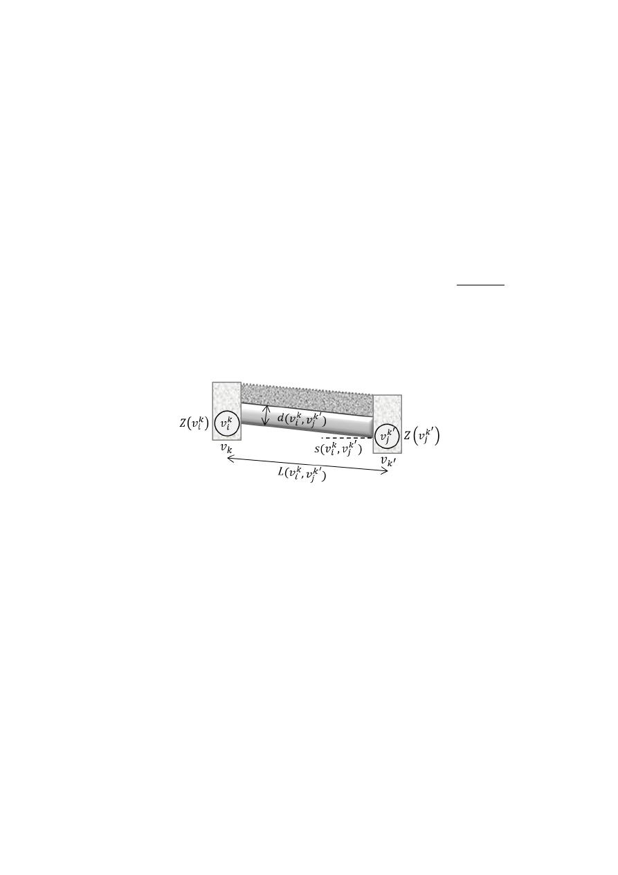
2
). Note that both diameter and invert elevations for every pipe
fully characterize a solution to the HD problem and, therefore, they represent the decision variables of
the problem. In our formulation of the problem, these decision variables are ultimately mapped to the
arcs in A
D
and their value is determined upon solving a shortest path problem as we explain next.
Water 2020, 12, x FOR PEER REVIEW
9 of 22
and 𝑍
denote the minimum and maximum invert elevations, respectively. Arc 𝑣 , 𝑣
represents a pipe from manhole 𝑙 to manhole 𝑙 with diameter 𝑑 𝑣 , 𝑣
= 𝛿 𝑣
and slope
𝑠 𝑣 , 𝑣
=
,
, where 𝐿 𝑣 , 𝑣
is the pipe length (Figure 2). Note that both diameter and
invert elevations for every pipe fully characterize a solution to the HD problem and, therefore, they
represent the decision variables of the problem. In our formulation of the problem, these decision
variables are ultimately mapped to the arcs in 𝒜 and their value is determined upon solving a
shortest path problem as we explain next.
Figure 2. Hydraulic design representation of a single pipeline (diameter-slope) [9].
By construction, 𝒢 ensures that basic hydraulic constraints are met. For instance, if water flows
from manhole 𝑙 towards manhole 𝑙 , only arcs satisfying a non-decreasing diameter and a positive
slope (in favour of gravity) exist. Formally, arc 𝑣 , 𝑣
is part of graph 𝒢 if and only if 𝛿 𝑣
≤
𝛿 𝑣
, 𝑠 𝑣 , 𝑣
> 0 , and all regulation-dependent constraints are satisfied. Note that typical
hydraulic constraints such as minimum and maximum depth, flow velocity, shear stress and quasi-
critical flow conditions, can be trivially evaluated for every arc 𝑣 , 𝑣
because all the required
input for the evaluation is known, i.e., diameter, slope, and flow rate (𝑄
).
Every arc in 𝒜 is equipped with a cost 𝐶 𝑣 , 𝑣
that represents the corresponding
construction cost (and potentially maintenance and operational cost). In our case studies we adopt
the cost function introduced by Li and Matthew [34], however, we emphasize that any cost function
can be employed. Similar to how our model trivializes the evaluation of hydraulic constraints, highly
non-linear cost functions are reduced to a parameter of the design graph. Most cost functions are
defined in terms of pipe diameter 𝑑 𝑣 , 𝑣
, pipe length 𝐿 𝑣 , 𝑣
, and average excavation depth
ℎ 𝑣 , 𝑣
= 0.5 ℎ 𝑣
− ℎ 𝑣
, where ℎ 𝑣 is the buried depth at the extreme of a pipe, i.e.,
ℎ 𝑣
= 𝑍 − 𝑍(𝑣 ).
To find an optimal hydraulic design for the given input layout, we solve a one-to-all shortest
path problem on 𝒢 starting from a dummy node 𝑣 that we connect to every node in 𝒩 (Figure
1). A solution to such a problem is a shortest path spanning tree 𝒫 rooted in 𝑣 . Formally, the
underlying optimization problem is defined by Equation (11).
min
𝒫
𝐶
𝑣 , 𝑣
𝑣
𝑖
𝑘
,𝑣
𝑗
𝑘′
∈𝒫
(11)
subject to 𝒫 being a shortest path spanning tree. The constraints that enforce 𝒫 to be a shortest path
spanning tree are omitted as we adopt an algorithmic approach to solve the problem instead of a
mathematical programming approach (as in the LS problem). A generic formulation of the SP
problem can be found in Ahuja et al. [39]. We use the Bellman–Ford algorithm [45] to optimally solve
problem 11. The Bellman–Ford algorithm relies on labels at each node that save the cumulative cost
from the starting node (𝑣 in our case). This label-correcting algorithm updates the cumulative cost
for each node when a least-cost label is found and saves its predecessor node [39]. When all the nodes
of the graph are evaluated, the cost labels are optimal. For more details about this algorithm, we refer
the reader to Duque et al. [9].
When different series of pipes in the network have a common pipe, the solution of the one-to-all
SP problem might include more than one arc between the manholes associated with the shared pipe.
Figure 2.
Hydraulic design representation of a single pipeline (diameter-slope) [
9
].
By construction, G
D
ensures that basic hydraulic constraints are met. For instance, if water flows
from manhole l
k
towards manhole l
k
0
, only arcs satisfying a non-decreasing diameter and a positive
slope (in favour of gravity) exist. Formally, arc
v
k
i
, v
k
0
j
is part of graph G
D
if and only if
δ
v
k
i
≤
δ
v
k
0
j
,
s
v
k
i
, v
k
0
j
> 0, and all regulation-dependent constraints are satisfied. Note that typical hydraulic
constraints such as minimum and maximum depth, flow velocity, shear stress and quasi-critical flow
conditions, can be trivially evaluated for every arc
v
k
i
, v
k
0
j
because all the required input for the
evaluation is known, i.e., diameter, slope, and flow rate (Q
kk
0
).
Every arc in A
D
is equipped with a cost C
v
k
i
, v
k
0
j
that represents the corresponding construction
cost (and potentially maintenance and operational cost). In our case studies we adopt the cost function
introduced by Li and Matthew [
34
], however, we emphasize that any cost function can be employed.
Similar to how our model trivializes the evaluation of hydraulic constraints, highly non-linear cost
functions are reduced to a parameter of the design graph. Most cost functions are defined in terms of pipe
diameter d
v
k
i
, v
k
0
j
, pipe length L
v
k
i
, v
k
0
j
, and average excavation depth h
v
k
i
, v
k
0
j
=
0.5
h
v
k
i
− h
v
k
0
j
,
where h
v
k
i
is the buried depth at the extreme of a pipe, i.e., h
v
k
i
=
Z
k
− Z
v
k
i
.
To find an optimal hydraulic design for the given input layout, we solve a one-to-all shortest
path problem on G
D
starting from a dummy node v
D
that we connect to every node in N
T
D
(Figure
1
).
Water 2020, 12, 3337
10 of 22
A solution to such a problem is a shortest path spanning tree P rooted in v
D
. Formally, the underlying
optimization problem is defined by Equation (11).
min
P
X
(v
k
i
,v
k
0
j
)∈P
C
v
k
i
, v
k
0
j
(11)
subject to P being a shortest path spanning tree. The constraints that enforce P to be a shortest path
spanning tree are omitted as we adopt an algorithmic approach to solve the problem instead of a
mathematical programming approach (as in the LS problem). A generic formulation of the SP problem
can be found in Ahuja et al. [
39
]. We use the Bellman–Ford algorithm [
45
] to optimally solve problem
11. The Bellman–Ford algorithm relies on labels at each node that save the cumulative cost from the
starting node (v
D
in our case). This label-correcting algorithm updates the cumulative cost for each
node when a least-cost label is found and saves its predecessor node [
39
]. When all the nodes of the
graph are evaluated, the cost labels are optimal. For more details about this algorithm, we refer the
reader to Duque et al. [
9
].
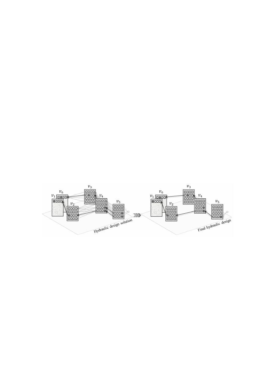
When di
fferent series of pipes in the network have a common pipe, the solution of the one-to-all
SP problem might include more than one arc between the manholes associated with the shared pipe.
If that is the case, the final design is adjusted by choosing the inner-branch pipe with lower invert
elevations (deeper pipe) and the largest diameter (e.g., pipe between tree layout nodes v
4
and v
5
in
Figure
3
). This adjustment ensures the design feasibility and does not compromise optimality since the
selected pipe (deepest and largest in diameter) also belongs to the optimal solution of the one-to-all SP
problem. The solution of this problem encodes the optimal hydraulic design of all the branches for a
fixed input layout.
Water 2020, 12, x FOR PEER REVIEW
10 of 22
If that is the case, the final design is adjusted by choosing the inner-branch pipe with lower invert
elevations (deeper pipe) and the largest diameter (e.g., pipe between tree layout nodes 𝑣 and 𝑣 in
Figure 3). This adjustment ensures the design feasibility and does not compromise optimality since
the selected pipe (deepest and largest in diameter) also belongs to the optimal solution of the one-to-
all SP problem. The solution of this problem encodes the optimal hydraulic design of all the branches
for a fixed input layout.
Figure 3. Selection of the definitive hydraulic design, eliminating double pipes generated from
different shortest paths.
The entire procedure for the hydraulic design is summarized as follows:
1.
Add a dummy design node 𝑣 connecting every design node in the outfall 𝒩 (see Figure 1);
2.
Assign a cost value 𝐶 𝑣 , 𝑣
for every arc in 𝒜 ;
3.
Reverse all arcs in 𝒜 and execute the Bellman–Ford algorithm [45] to obtain the one-to-all
shortest paths from the outfall node 𝑣 to every other node in 𝒩 ;
4.
Retrieve the best paths from 𝑣 to any design node in 𝒩 ∀ 𝑣 ∈ 𝒩 ;
5.
Select the deepest and largest diameter pipe when multiple design arcs 𝑣 , 𝑣
∈ 𝒜 that are
part of different shortest paths belong to the same tree arc (𝑣 , 𝑣 ) ∈ 𝒜 , since only one pipe
should exist in each section.
3.4. Iterative Scheme
We conclude our methodological section with a description of the iterative scheme and an
outline of the entire algorithm. As mentioned, during a single iteration the LS and HD problems are
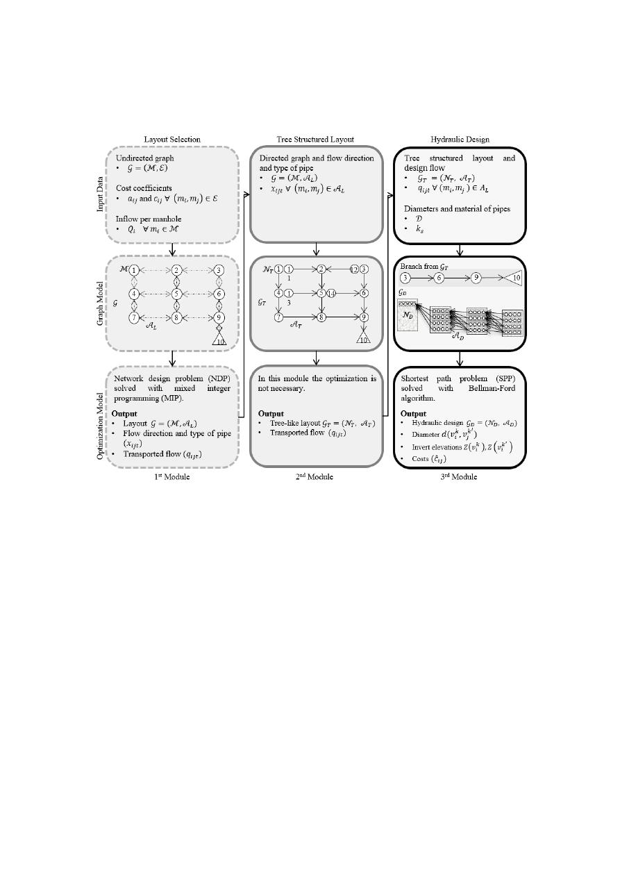
solved in a sequential manner. Figure 4 summarizes the three modules and modelling frameworks
for a single iteration.
Figure 3.
Selection of the definitive hydraulic design, eliminating double pipes generated from di
fferent
shortest paths.
The entire procedure for the hydraulic design is summarized as follows:
1.
Add a dummy design node v
D
connecting every design node in the outfall N
T
D
(see Figure
1
);
2.
Assign a cost value C
v
k
i
, v
k
0
j
for every arc in A
D
;
3.
Reverse all arcs in A
D
and execute the Bellman–Ford algorithm [
45
] to obtain the one-to-all
shortest paths from the outfall node v
D
to every other node in N
D
;
4.
Retrieve the best paths from v
D
to any design node in N
k
D
∀ v
k
∈ N
T
;
5.
Select the deepest and largest diameter pipe when multiple design arcs
v
k
i
, v
k
0
j
∈ A
D
that are
part of di
fferent shortest paths belong to the same tree arc
(
v
k
, v
k
0
)
∈ A
T
, since only one pipe
should exist in each section.
3.4. Iterative Scheme
We conclude our methodological section with a description of the iterative scheme and an outline
of the entire algorithm. As mentioned, during a single iteration the LS and HD problems are solved
Water 2020, 12, 3337
11 of 22
in a sequential manner. Figure
4
summarizes the three modules and modelling frameworks for a
single iteration.
Water 2020, 12, x FOR PEER REVIEW
11 of 22
Figure 4. Sewer networks design (SND) modules and modelling frameworks for a single iteration.
Recall that the cost of a sewer network is a function of the diameter, length, and excavation
volume of each pipe. However, diameters and excavation volumes are not decision variables of the
LS problem and therefore the objective function (Equation (1)) approximates the hydraulic design
cost as a function of the flow rates 𝐪 and the flow direction 𝐱. Equation (1) implies a linear model to
approximate the cost of a pipe from manhole 𝑚 to manhole 𝑚 , as a function of 𝑞 and 𝑥 . Let
𝑐̂ be a prediction of the cost of a pipe from 𝑚 to 𝑚 under the linear model in Equation (12).
𝑐̂ = 𝑐 𝑞 + 𝑎 𝑥
(12)
Our goal is to estimate parameters 𝑐 and 𝑎 for all 𝑚 , 𝑚
∈ 𝒜 as a new input to the LS
problem. We estimate 𝑐 and 𝑎 independently for each arc by means of linear regression. For a
particular arc 𝑚 , 𝑚 , we regress previous values 𝑞 and 𝑥 against the cost obtained in the
hydraulic design for this pair of manholes, i.e., 𝐶(𝑣, 𝑣 ) for some arc (𝑣, 𝑣 ) ∈ 𝒫 that belongs to the
shortest path spanning tree for which nodes 𝑣 and 𝑣 are associated to manholes 𝑚 and 𝑚 ,
respectively. Note that indices for 𝑣 and 𝑣 were dropped to avoid cumbersome notation. As the
algorithm progresses, we obtain new observations of 𝑐̂ , 𝑞 , and 𝑥 that refine the estimation of
the parameters. Refining the estimation ultimately improves the prediction of the cost and, therefore,
the quality of subsequent layouts.
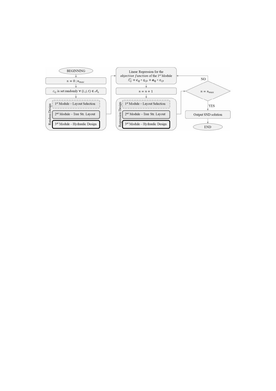
Figure 5 presents the entire framework in a flow diagram. We start with an initialization
procedure that generates a hydraulic design based on a randomized layout. This step is necessary to
obtain the observations for the parameter estimation in the regression step. The randomized layouts
are obtained by simply assigning random values to 𝑐 and 𝑎 and solving the MIP model. In the
iterative phase, the algorithm executes the three modules described above until a maximum number
of iterations is met. After each iteration, the linear regression considers all the costs obtained from the
hydraulic designs, providing a better estimate of the LS cost coefficients 𝑐 and 𝑎 .
Figure 4.
Sewer networks design (SND) modules and modelling frameworks for a single iteration.
Recall that the cost of a sewer network is a function of the diameter, length, and excavation volume
of each pipe. However, diameters and excavation volumes are not decision variables of the LS problem
and therefore the objective function (Equation (1)) approximates the hydraulic design cost as a function
of the flow rates q and the flow direction x. Equation (1) implies a linear model to approximate the
cost of a pipe from manhole m
i
to manhole m
j
, as a function of q
i jt
and x
i jt
. Let ˆc
i j
be a prediction of the
cost of a pipe from m
i
to m
j
under the linear model in Equation (12).
ˆc
i j
=
c
i j
q
i jt
+
a
i j
x
i jt
(12)
Our goal is to estimate parameters c
i j
and a
i j
for all
m
i
, m
j
∈ A
L
as a new input to the LS problem.
We estimate c
i j
and a
i j
independently for each arc by means of linear regression. For a particular arc
m
i
, m
j
, we regress previous values ˆq
i jt
and ˆx
i jt
against the cost obtained in the hydraulic design for
this pair of manholes, i.e., C
(
v, v
0
)
for some arc
(
v, v
0
)
∈ P that belongs to the shortest path spanning
tree for which nodes v and v
0
are associated to manholes m
i
and m
j
, respectively. Note that indices for
v and v
0
were dropped to avoid cumbersome notation. As the algorithm progresses, we obtain new
observations of ˆc
i j
, q
i jt
, and x
i jt
that refine the estimation of the parameters. Refining the estimation
ultimately improves the prediction of the cost and, therefore, the quality of subsequent layouts.
Figure
5
presents the entire framework in a flow diagram. We start with an initialization procedure
that generates a hydraulic design based on a randomized layout. This step is necessary to obtain the
observations for the parameter estimation in the regression step. The randomized layouts are obtained
by simply assigning random values to c
i j
and a
i j
and solving the MIP model. In the iterative phase,
Water 2020, 12, 3337
12 of 22
the algorithm executes the three modules described above until a maximum number of iterations is
met. After each iteration, the linear regression considers all the costs obtained from the hydraulic
designs, providing a better estimate of the LS cost coe
fficients c
i j
and a
i j
.
Water 2020, 12, x FOR PEER REVIEW
12 of 22
Figure 5. Sewer networks design (SND) problem flow chart.
3.5. Software and Data
The SND framework is mainly coded in Java. The layout selection module, however, is coded in
Mosel, which is a mathematical modelling and programming language to model the MIP problem
[43]. The SND software is available to download from
https://bitbucket.org/nduquevillarreal/snd_java-xpress.git. It was designed to have few data
requirements for the design of sewer systems. We provide the input data of our case studies in the
Supplementary Material.
3.6. Case Studies
To compare our approach to others found in the literature, we tested our methodology on two
benchmark networks. The first benchmark, proposed by Li and Matthew [34], has 79 pipes and 78
manholes and has been used over the years by several authors to test their algorithms [4,12,46,47].
The second benchmark network proposed by Moeini and Afshar [31], has 81 manholes and 144 pipes.
In addition, we also tested our methodology in a network that is part of the real sewer network in
Bogota, Colombia. This network, labelled Chicó, has 109 manholes, 160 pipes with lengths between
65 m and 204 m, steep ground and a total flow of 1.526 m
3
/s. For the hydraulic design of these
networks, we used the cost function, design parameters and constraints proposed by Li and Matthew
[34]. Table 1 presents the hydraulic constraints and Equations (13) and (14) present the construction
costs for a pipe 𝑓 and a manhole 𝑓 , respectively [34].
Table 1. Hydraulic design constraints for round pipes [34].
Constraint Value
Condition
1
Minimum diameter
0.2 m
Always
2 Maximum
filling
ratio
0.6
𝑑 ≤ 0.3 m
0.7
0.35 ≤ 𝑑 ≤ 0.45 m
0.75
0.50 ≤ 𝑑 ≤ 0.90 m
0.8
𝑑 ≥ 1.0 m
3 Minimum
velocity
0.7 m/s
𝑑 ≤ 0.5 m
0.8m/s
𝑑 > 0.5 m
4 Maximum
velocity 5.0
m/s
5
Minimum gradient
0.003
Flow rate < 0.015 m /s
𝑓 =
⎝
⎜
⎛(4.27 + 93.59𝑑 + 2.86𝑑ℎ + 2.39ℎ )𝐿 𝑤𝑖𝑡ℎ 𝑑 ≤ 1 𝑚 𝑎𝑛𝑑 ℎ ≤ 3 𝑚
(36.47 + 88.96𝑑 + 8.70𝑑ℎ + 1.78ℎ )𝐿 𝑤𝑖𝑡ℎ 𝑑 ≤ 1 𝑚 𝑎𝑛𝑑 ℎ > 3 𝑚
(20.50 + 149.27𝑑 − 58.96𝑑ℎ + 17.75ℎ )𝐿 𝑤𝑖𝑡ℎ 𝑑 > 1 𝑚 𝑎𝑛𝑑 ℎ ≤ 4 𝑚
(78.44 + 29.25𝑑 + 31.80𝑑ℎ − 2.32ℎ )𝐿 𝑤𝑖𝑡ℎ 𝑑 > 1 𝑚 𝑎𝑛𝑑 ℎ > 4 𝑚⎠
⎟
⎞
(13)
Figure 5.
Sewer networks design (SND) problem flow chart.
3.5. Software and Data
The SND framework is mainly coded in Java. The layout selection module, however, is coded in
Mosel, which is a mathematical modelling and programming language to model the MIP problem [
43
].
The SND software is available to download from
https:
//bitbucket.org/nduquevillarreal/snd_java-
xpress.git
. It was designed to have few data requirements for the design of sewer systems. We provide
the input data of our case studies in the Supplementary Material.
3.6. Case Studies
To compare our approach to others found in the literature, we tested our methodology on two
benchmark networks. The first benchmark, proposed by Li and Matthew [
34
], has 79 pipes and
78 manholes and has been used over the years by several authors to test their algorithms [
4
,
12
,
46
,
47
].
The second benchmark network proposed by Moeini and Afshar [
31
], has 81 manholes and 144 pipes.
In addition, we also tested our methodology in a network that is part of the real sewer network in
Bogota, Colombia. This network, labelled Chicó, has 109 manholes, 160 pipes with lengths between
65 m and 204 m, steep ground and a total flow of 1.526 m
3
/s. For the hydraulic design of these networks,
we used the cost function, design parameters and constraints proposed by Li and Matthew [
34
]. Table
1
presents the hydraulic constraints and Equations (13) and (14) present the construction costs for a pipe
f
p
and a manhole f
m
, respectively [
34
].
f
p
=
4.27
+
93.59d
2
+
2.86dh
+
2.39h
2
L
with d ≤ 1 m and h ≤ 3 m
36.47
+
88.96d
2
+
8.70dh
+
1.78h
2
L
with d ≤ 1 m and h
> 3 m
20.50
+
149.27d
2
− 58.96dh
+
17.75h
2
L
with d
> 1 m and h ≤ 4 m
78.44
+
29.25d
2
+
31.80dh − 2.32h
2
L
with d
> 1 m and h > 4 m
(13)
f
m
=
136.67
+
166.19d
2
+
3.5dh
+
16.22h
2
with d ≤ 1 m and h ≤ 3 m
132.91
+
790.94d
2
− 280.23dh
+
34.97h
2
with d ≤ 1 m and h
> 3 m
209.74
+
57.53d
2
+
10.93dh
+
19.88h
2
with d
> 1 m and h ≤ 3 m
210.66 − 113.04d
2
+
126.43dh − 0.60h
2
with d
> 1 m and h > 3 m
(14)

Water 2020, 12, 3337
13 of 22
Table 1.
Hydraulic design constraints for round pipes [
34
].
Constraint
Value
Condition
1
Minimum diameter
0.2 m
Always
2
Maximum filling
ratio
0.6
d ≤ 0.3 m
0.7
0.35 ≤ d ≤ 0.45 m
0.75
0.50 ≤ d ≤ 0.90 m
0.8
d ≥ 1.0 m
3
Minimum velocity
0.7 m/s
d ≤ 0.5 m
0.8 m/s
d
> 0.5 m
4
Maximum velocity
5.0 m/s
5
Minimum gradient
0.003
Flow rate
< 0.015 m
3
/s
The variables f
p
and f
m
are calculated in terms of the pipe diameter d, the length L, and average
buried depth h. The network construction cost is the sum of all costs of pipes and manholes in
the network. Annual maintenance cost is 4.2% of the construction cost, considered for a 10-year
period [
34
]. Construction and operational costs of pumping are not considered since our design
considers gravity-driven systems. Additionally, we used concrete pipes (Manning coe
fficient n = 0.014
and the following list of diameters: {0.2, 0.25, 0.3, 0.35, 0.38, 0.4, 0.45, 0.5, 0.53, 0.6, 0.7, 0.8, 0.9, 1.0, 1.05,
1.20, 1.35, 1.4, 1.5, 1.6, 1.8, 2, 2.2, 2.4}.
The input data and detailed results for all networks can be found in the Supplementary Material
and the Git repository. The input data includes the Id of the manholes and pipes, inflow Q
i
in [m
3
/s]
and the x, y and z coordinates in [m] at each manhole. The results for the hydraulic design for each
pipe include upstream and downstream manhole, type [inner
/outer], diameter [m], upstream and
downstream invert elevation [m], flow rate [m
3
/s] and slope [–].
4. Results
4.1. Benchmark Li and Matthew
After 10 iterations using an elevation change of
∆Z = 0.1 m, the hydraulic design for this layout
costs ¥ 1.33 × 10
6
and has a maintenance cost of ¥ 0.55 × 10
6
. The design has a maximum excavation
depth of 9.45 m, and took a computational time of 45 min to solve both the LS and HD. An additional
iteration was done to design the same layout with higher precision (i.e., a finer elevation change
of
∆Z = 0.01 m). Figure
6
shows the layout and hydraulic design obtained using
∆Z = 0.01 m.
The construction and maintenance costs were reduced to ¥ 1.29 × 10
6
and ¥ 0.54 × 10
6
, respectively.
For this design, we obtained a maximum excavation depth of 9.38 m and a computational time of
58 min for a single iteration of the hydraulic design. The detailed hydraulic design can be found in the
Supplementary Material.
Table
2
shows a comparison of the results found in the literature for the network design proposed
by Li and Matthew [
34
], which do not include pumping. All the authors presented in this table use the
same constraints (Table
1
) and cost functions comprising pipe f
p
and manhole f
m
costs (Equations (13)
and (14)) [
34
]. We compare results obtained using di
fferent optimization approaches for cases where
the layout is taken by Li and Matthew [
34
] and only the hydraulic design is optimized [
4
,
12
,
46
,
47
]
and where, as for the present work, both layout and hydraulic design are optimized [
20
,
28
,
31
,
48
].
Our methodology obtained the lowest cost after 10 iterations with a modest computational time.
Water 2020, 12, 3337
14 of 22
Water 2020, 12, x FOR PEER REVIEW
14 of 22
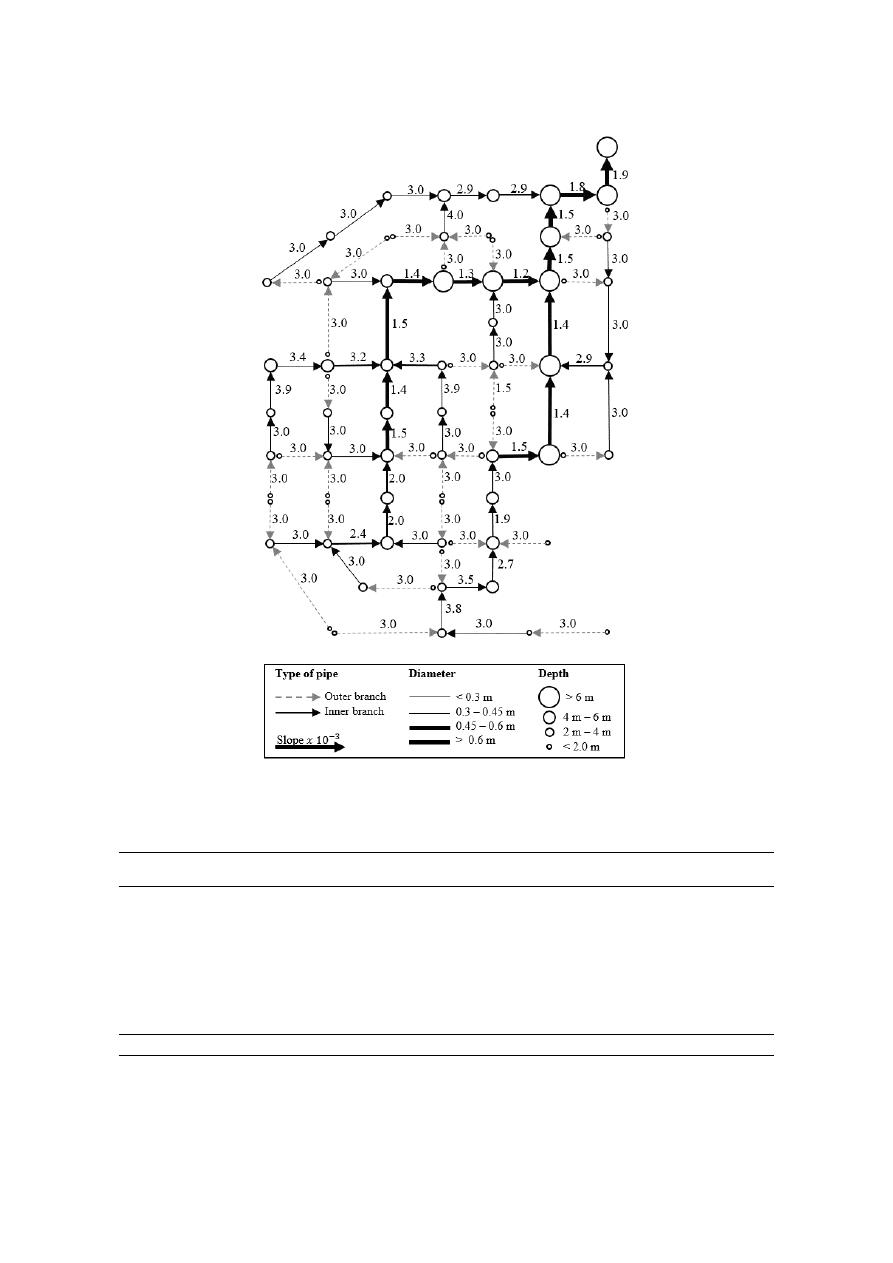
Figure 6. Layout and hydraulic design (∆Z = 0.01 m) of the benchmark proposed by Li and Matthew
[34], using the proposed methodology.
Table 2 shows a comparison of the results found in the literature for the network design
proposed by Li and Matthew [34], which do not include pumping. All the authors presented in this
table use the same constraints (Table 1) and cost functions comprising pipe 𝑓 and manhole 𝑓 costs
(Equations (13) and (14)) [34]. We compare results obtained using different optimization approaches
for cases where the layout is taken by Li and Matthew [34] and only the hydraulic design is optimized
[4,12,46,47] and where, as for the present work, both layout and hydraulic design are optimized
[20,28,31,48]. Our methodology obtained the lowest cost after 10 iterations with a modest
computational time.
Table 2. Comparison of the construction cost for the benchmark proposed by Li and Matthew [34].
Method Researchers
Optimized
Layout
Construction Cost
(Yuan) × 10
6
MGA
Pan and Kao [46]
No
¥ 1.91
Adaptive GA
Haghighi and Bakhshipour [12]
No
¥ 1.84
MILP
Safavi and Geranmehr [4]
No
¥ 1.57
SDE-GOBL
Liu et al. [47]
No
¥ 1.53
Figure 6.
Layout and hydraulic design (
∆Z = 0.01 m) of the benchmark proposed by Li and Matthew [
34
],
using the proposed methodology.
Table 2.
Comparison of the construction cost for the benchmark proposed by Li and Matthew [
34
].
Method
Researchers
Optimized Layout
Construction Cost
(Yuan) × 10
6
MGA
Pan and Kao [
46
]
No
Y = 1.91
Adaptive GA
Haghighi and Bakhshipour [
12
]
No
Y = 1.84
MILP
Safavi and Geranmehr [
4
]
No
Y = 1.57
SDE-GOBL
Liu et al. [
47
]
No
Y = 1.53
Loop-by-loop cutting algorithm
and GA-DDDP
Haghighi and Bakhshipour [
28
]
Yes
Y = 1.59
Loop-by-loop cutting algorithm
and TS
Haghighi and Bakhshipour [
20
]
Yes
Y = 1.43
Reliability - DDDP
Haghighi and Bakhshipour [
48
]
Yes
Y = 2.41
ACOA-TGA-NLP
Moeini and Afshar [
31
]
Yes
Y = 1.39
MIP and DP
(Present work)
Yes
Y = 1.29
Our layout could be improved with more iterations to gain a better approximation of the costs in
terms of the flow and pipe direction. A non-linear cost approximation for the LS problem could also
improve the results of the layout and, therefore, the entire sewer network design algorithm.

Water 2020, 12, 3337
15 of 22
4.2. Benchmark Moeini and Afshar
We obtained a design for the benchmark network studied in Moeini and Afshar [
31
] that attains
a total cost of ¥ 524,687 after 30 iterations of the algorithm, using an elevation change of
∆Z = 0.1 m.
Additionally, we conducted an experiment in which the layout is fixed to that of Moeini and Afshar [
31
]
and solved only the hydraulic design problem. This design costs ¥ 569,334, using the same elevation
change of
∆Z = 0.1 m. Both scenarios assume the same constraints, cost function and conditions
described in Li and Matthew [
34
]. Total costs include the construction costs and maintenance costs
(Table
3
). Column 1 describes the statistics of interest; column 2 shows the results reported in Moeini
and Afshar [
31
], column 3 shows the results when we only apply the HD component of our algorithm on
the layout reported by Moeini and Afshar [
31
]; and finally, column 4 shows the results of our algorithm.
Table 3.
Comparison of the total cost for the benchmark proposed by Moeini and Afshar [
31
].
ACOA-TGA-NLP [
31
]
DP (Present work) with
Fixed Layout [
31
]
MIP and DP
(Present Work)
Costs
Construction Cost
¥ 640,845 *
¥ 400,940
¥ 369,498
Maintenance Cost
¥ 269,155 *
¥ 168,395
¥ 155,189
Total Cost
¥ 910,000 *
¥ 569,335
¥ 524,687
Computational e
ffort
Iterations [–]
10
1
30
Time [min]
198
4
115
Physical characteristics
Average diameter [m]
0.331 **
0.262
0.267
Average depth [m]
Not reported
2.07
1.95
Outfall diameter [m]
1.05 **
0.7
0.8
Outfall depth [m]
Not reported
6.6
5.4
* Estimated from the reported total cost. ** Based on the reported design solution [
31
].
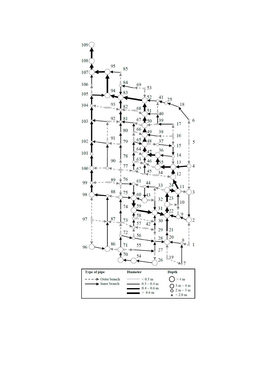
4.3. Real Network: Chicó
Figure
7
shows the layout obtained after 25 iterations using an elevation change of
∆Z = 0.1 m.
The hydraulic design for this layout uses the same constraints, cost function and conditions described in
Li and Matthew [
34
]. The construction and maintenance costs are ¥ 699,097 and ¥ 293,621, respectively.
Therefore, the total cost is ¥ 992,718. The design has a maximum excavation depth of 15.9 m and a
diameter in the outfall of 1.05 m. All iterations took a computational time of 113 min to solve both the
LS and HD. The detailed hydraulic design can be found in the Supplementary Material as well as the
distribution of the coe
fficient of determination R
2
of the linear approximation of the cost function for
each pipe after 25 iterations. The average R
2
is 0.84, with a standard deviation of 0.23. The R
2
across all
the individual linear regressions varied from a minimum of 0.004 and a maximum of 1. Pipes with
R
2
= 1 represent those pipes that had the exact same design along the iterations.
4.4. Convergence Curves
We close this section with a convergence analysis of the algorithm. For each case study, Figure
8
shows the construction cost of the sewer network design obtained at each iteration of our algorithm.
Our algorithm behaves somewhat similarly across the three case studies. The first design leads to a
relatively high cost due to a poor initial layout that is obtained with random coe
fficients in Equation (1).
However, all subsequent iterations benefit from the cost function approximation that is employed in
the LS problem. Moreover, as the algorithm progresses, the cost function approximation is refined
with new hydraulic design solutions that populate the linear regression. In short, these convergence
curves highlight a core component of our framework that enables the HD problem to provide feedback
to the LS problem.
Water 2020, 12, 3337
16 of 22
Water 2020, 12, x FOR PEER REVIEW
16 of 22
solve both the LS and HD. The detailed hydraulic design can be found in the Supplementary Material.
as well as the distribution of the coefficient of determination R
2
of the linear approximation of the
cost function for each pipe after 25 iterations. The average R
2
is 0.84, with a standard deviation of
0.23. The R
2
across all the individual linear regressions varied from a minimum of 0.004 and a
maximum of 1. Pipes with R
2
= 1 represent those pipes that had the exact same design along the
iterations.
Figure 7. Layout and hydraulic design of Chicó sewer network.
Figure 7.
Layout and hydraulic design of Chicó sewer network.
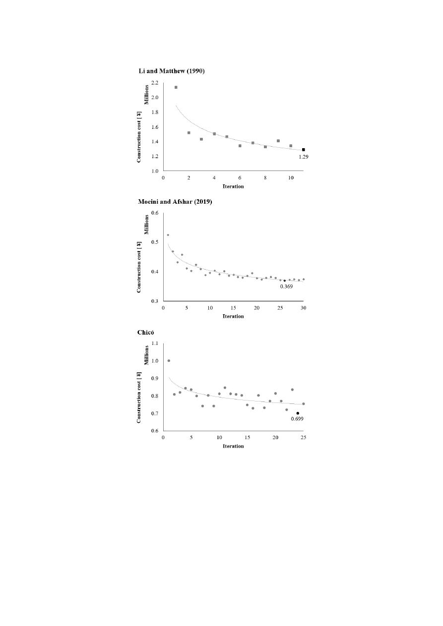
Water 2020, 12, 3337
17 of 22
Water 2020, 12, x FOR PEER REVIEW
17 of 22
4.4. Convergence Curves
We close this section with a convergence analysis of the algorithm. For each case study, Figure
8 shows the construction cost of the sewer network design obtained at each iteration of our algorithm.
Our algorithm behaves somewhat similarly across the three case studies. The first design leads to a
relatively high cost due to a poor initial layout that is obtained with random coefficients in Equation
(1). However, all subsequent iterations benefit from the cost function approximation that is employed
in the LS problem. Moreover, as the algorithm progresses, the cost function approximation is refined
with new hydraulic design solutions that populate the linear regression. In short, these convergence
curves highlight a core component of our framework that enables the HD problem to provide
feedback to the LS problem.
Figure 8. Convergence curves for each case study concerning construction costs.
Figure 8.
Convergence curves for each case study concerning construction costs.
5. Discussion
For all case studies, the proposed methodology found a better solution than those reported in the
literature. These are near-optimal solutions with respect to construction cost that satisfy all hydraulic
constraints and ensure feasible pipe connections in a sewer system. The LS is modelled as an MIP and
is solved exactly (for a particular objective function approximation) with an o
ff-the-shelf optimization
solver. The cost function approximation for the LS problem is enhanced by the results of new hydraulic
designs, as shown with the convergence curves in Figure
8
. Hydraulic design solutions of previous
iterations are used as additional data points in a linear regression model that estimates construction
costs as a linear function of the flow rate and the flow direction. These solutions are not intended
to be the global optimal solution for the network design, since the layout selection problem uses a

Water 2020, 12, 3337
18 of 22
proxy for construction costs that might not be the best approximation of the cost. Nevertheless, once a
near-optimal layout is selected, we obtained an optimal hydraulic design for the specific near-optimal
layout. As expected, during the first iterations, there is a big improvement of the LS cost function
and then the algorithms start to converge to a constant value. The minimum cost hydraulic design
represents the best layout obtained for that network within the number of iterations or accepted
tolerance for the design.
The comparison of all the results obtained by di
fferent authors (Table
2
) over the well-known
benchmark proposed by Li and Matthew [
34
] shows that our methodology obtains the best cost, even if
the layout optimization is not optimal. Some authors used the exact same layout proposed by Li and
Matthew [
34
] and only solved the hydraulic design problem with the best result cost ¥ 1.53 × 10
6
using
the self-adaptive di
fferential evolution algorithm [
47
]. Later researchers tackled the LS problem as
well, aiming for better results for the final hydraulic design. Previously, the best solution for both the
LS and HD problems cost ¥ 1.39 × 10
6
using ACOA-TGA-NLP [
31
]. Our methodology shows a big
improvement by saving up to 16% of the costs compared to the lowest cost found in the literature,
with a final cost of ¥ 1.29 × 10
6
.
Regarding the results for the second benchmark proposed by Moeini and Afshar [
31
] presented
in Table
3
, we obtained up to 37% savings on the HD using Moeini and Afshar’s layout, and up to
42% savings when solving both the LS and HD with our approach. As expected, we have a high
computational e
ffort given that our methodology makes an exhaustive search among all possible
design combinations. Nonetheless, the computational time spent by our algorithm was lower than the
result obtained using ACOA-TGA-NLP [
31
]. Therefore, we can say that our computational time is
acceptable considering the improvement we obtain in the total construction cost. The last case study
was proposed as a new benchmark using a network with real topographic data with mild slopes.
Our methodology can be improved by getting a better proxy for the cost function used to solve
the LS problem. The current cost function is obtained through a linear regression of previous design
options for the network. A non-linear cost approximation for the LS problem could also improve the
results of the layout and, therefore, the entire sewer network design algorithm. This improvement
might also have a positive impact on the computational time required to obtain a near-optimal sewer
network design.
6. Conclusions
We proposed a mathematical optimization framework for the design of sewer networks, with the
objective of minimizing construction costs while ensuring proper performance of the sewer network.
A graph modelling framework was proposed to represent the di
fferent features of a sewer network
design. The layout selection graph (Figure
1
) represents the type and flow direction of each pipe
that are the decision variables for the LS problem. A second graph represents the layout as an open
network, with a tree structure that avoids loops. The last graph represents the hydraulic design
problem, modelling the diameters and invert elevations of the pipes.
The LS is modelled as an MIP, which is solved for a particular objective function with an
o
ff-the-shelf optimization solver. The objective function approximation is enhanced by new hydraulic
design solutions, which are used as additional data points in a linear regression model that estimates
construction costs as a linear function of the flow rate and the flow direction. On the other hand,
the extension of the hydraulic design methodology proposed by Duque et al. [
9
] ensures the global
optimal hydraulic design for the given layout and design conditions. The iterative scheme significantly
reduces construction costs during the first iterations and it encounters a near-optimal solution as the
algorithm progresses. Better approximations of the real cost function for the layout selection model
might translate into further improvement of the overall design. Moreover, the method can be extended
to consider pumping stations for flat terrain by using additional arcs in the design graph.
Since the size of the problem increases exponentially with the number of pipes in the network,
there is a computational capacity burden in that fewer iterations can be executed for large-scale

Water 2020, 12, 3337
19 of 22
networks. Future research is needed to formulate better cost function approximations for the layout
selection (e.g., non-linear functions) to produce a better representation of the construction cost in this
stage of the design. Furthermore, our methodology could leverage parallel computing to speed up
certain components of the framework such as the hydraulic design.
Supplementary Materials:
The following are available online at
http:
//www.mdpi.com/2073-4441/12/12/3337/s1
,
Table S1: Input data Benchmark proposed by Li and Matthew [
34
]. The exact x and y coordinates are not defined,
however the length of the pipes is known, Table S2: Hydraulic design for the Benchmark proposed by Li and
Matthew [
34
], Table S3: Input data Benchmark proposed by Moeini and Afshar [
31
], Table S4: Hydraulic design for
the Benchmark proposed by Moeini and Afshar [
31
], Table S5: Input data for the manholes of Chicó’s sewer network
(109 manholes), Table S6: Hydraulic design for the Benchmark Chicó, Figure S1: Coe
fficient of determination R
2
of the linear approximation of the cost function for each pipe in Chicó case study after 25 iterations, Figure S2:
Global fitness of the linear approximation of the cost in terms of the flow rate.
Author Contributions:
Conceptualization, N.D., D.D. and J.S.; Software, N.D. and D.D.; Validation, N.D. and
A.A.; Formal Analysis, N.D., D.D., A.A. and J.S.; Writing—Original Draft Preparation, N.D., D.D., A.A. and J.S.;
Writing—Review and Editing, N.D., D.D., A.A. and J.S. All authors have read and agreed to the published version
of the manuscript.
Funding:
This research received no external funding.
Acknowledgments:
The authors would like to thank Diego Alejandro Paez from Queen’s University, Kingston,
Canada for his valuable feedback on the mathematical formulation for the layout selection model. We also
thank Mariane Schneider from Eawag
/ETH Zürich, and Peter M. Bach, postdoctoral fellow at Eawag, for their
valuable comments that significantly improved the paper. The authors thank two anonymous referees for helpful
suggestions, which improved the paper.
Conflicts of Interest:
The authors declare no conflict of interest.
Nomenclature
Layout Selection
G
is the graph that represents the layout selection problem.
M
is the set of nodes representing manholes.
E
is the set of undirected edges representing links between two nodes m
i
∈ M and
m
j
∈ M.
Q
i
is the inflow at manhole m
i
∈ M.
Q
K
is the total flow in the system reaching the outfall manhole m
k
∈ M .
Z
i
is the ground elevation at manhole m
i
∈ M.
T
is the set of possible types of pipes, containing outer-branch pipes (t
1
) and
inner-branch pipes (t
2
).
A
L
is the set of directed links between two manholes, m
i
and m
j
, so that
m
i
, m
j
∈ E.
x
i jt
is the binary decision variable that represents the flow direction and
connection type in the network layout, for all
m
i
, m
j
∈ A
L
and t ∈ T .
q
i jt
is the continuous decision variable that represents the flow through arc
(
m
i
, m
j
)
of
type t, for all
m
i
, m
j
∈ A
L
and t ∈ T .
M
is a large positive number.
Tree-structured Layout
G
T
is the graph that represents the selected layout as a tree-structured network.
N
T
is the set of nodes in the tree-structured graph G
T
.
l
k
is a label that represents the index of the manhole associated to tree node v
k
∈ N
T
N
i
T
is a subset of N
T
that contains tree nodes associated with manhole m
i
∈ M.
A
T
is the set of arcs in the tree-structured graph G
T
.
Hydraulic Design
G
D
is the auxiliary graph used to represent the hydraulic design problem.
N
D
is the set of nodes in the hydraulic design graph G
D
, which is divided in subsets
of nodes N
k
D
related with the tree node v
k
∈ N
T
.
A
D
is the set of arcs of the hydraulic design graph G
D
.
D
is the discrete set of commercially available pipe diameters.

Water 2020, 12, 3337
20 of 22
δ
v
k
i
is the discrete decision variable that represents a possible diameter for an
upstream pipe of tree node v
k
∈ N
T
and manhole l
k
.
Z
v
k
i
is the continuous decision variable that represents the elevation above a reference
level of a node of the graph G
D
.
s
is the slope for each pipe, fully determined by the invert elevations Z
v
k
i
and
Z
v
k
j
at the extremes of the arc
v
k
i
, v
k
0
j
∈ A
D
which represents a pipe.
k
s
is the absolute roughness of the pipes.
References
1.
Elimam, A.A.; Charalambous, C.; Ghobrial, F.H. Optimum design of large sewer networks. J. Environ. Eng.
1989
, 115, 1171–1190. [
CrossRef
]
2.
Swamee, P.K.; Sharma, A.K. Optimal design of a sewer line using linear programming. Appl. Math. Model.
2013
, 37, 4430–4439. [
CrossRef
]
3.
Gupta, M.; Rao, P.; Jayakumar, K. Optimization of integrated sewerage system by using simplex method.
VFSTR J. STEM 2017, 3, 2455-2062.
4.
Safavi, H.; Geranmehr, M.A. Optimization of sewer networks using the mixed-integer linear programming.
Urban Water J. 2017, 14, 452–459. [
CrossRef
]
5.
Holland, M.E. Computer Models of Waste-Water Collection Systems. Ph.D. Thesis, Harvard University,
Cambridge, MA, USA, May 1966.
6.
Mansouri, M.;
Khanjani, M. Optimization of sewer networks using nonlinear programming.
J. Water Wastewater. 1999, 10, 20–30.
7.
Mays, L.W.; Yen, B.C. Optimal cost design of branched sewer systems. Water Resour. Res. 1975, 11, 37–47.
[
CrossRef
]
8.
Walters, G.A. The design of the optimal layout for a sewer network. Eng. Optim. 1985, 9, 37–50. [
CrossRef
]
9.
Duque, N.; Duque, D.; Saldarriaga, J. A new methodology for the optimal design of series of pipes in sewer
systems. J. Hydroinf. 2016, 18, 757–772. [
CrossRef
]
10.
Kulkarni, V.S.; Khanna, P. Pumped wastewater collection systems optimization. J. Environ. Eng. 1985,
111, 589–601. [
CrossRef
]
11.
Afshar, M.H. Rebirthing genetic algorithm for storm sewer network design. Sci. Iran. 2012, 19, 11–19.
[
CrossRef
]
12.
Haghighi, A.; Bakhshipour, A.E. Optimization of sewer networks using an adaptive genetic algorithm.
Water Resour. Manag. 2012, 26, 3441–3456. [
CrossRef
]
13.
Palumbo, A.; Cimorelli, L.; Covelli, C.; Cozzolino, L.; Mucherino, C.; Pianese, D. Optimal design of urban
drainage networks. Civ. Eng. Environ. Syst. 2014, 31, 79–96. [
CrossRef
]
14.
Cozzolino, L.; Cimorelli, L.; Covelli, C.; Mucherino, C.; Pianese, D. An innovative approach for drainage
network sizing. Water 2015, 7, 546–567. [
CrossRef
]
15.
Cisty, M. Hybrid genetic algorithm and linear programming method for least-cost design of water distribution
systems. Water Resour. Manag. 2010, 24, 1–24. [
CrossRef
]
16.
Hassan, W.H.; Jassem, M.H.; Mohammed, S.S. A GA-HP model for the optimal design of sewer networks.
Water Resour. Manag. 2018, 32, 865–879. [
CrossRef
]
17.
Afshar, M.H. A parameter free continuous ant colony optimization algorithm for the optimal design of storm
sewer networks: Constrained and unconstrained approach. Adv. Eng. Softw. 2010, 41, 188–195. [
CrossRef
]
18.
Moeini, R.; Afshar, M.H. Arc based ant colony optimization algorithm for optimal design of gravitational
sewer networks. Ain Shams Eng. J. 2017, 8, 207–223. [
CrossRef
]
19.
Yeh, S.F.; Chang, Y.J.; Lin, M.D. Optimal design of sewer network by tabu search and simulated annealing.
In Proceedings of the 2013 IEEE International Conference on Industrial Engineering and Engineering
Management, Bangkok, Thailand, 10–13 December 2013; Institute of Electrical and Electronics Engineers
(IEEE): Piscataway, NJ, USA, 2013; pp. 1636–1640.
20.
Haghighi, A.; Bakhshipour, A.E. Deterministic integrated optimization model for sewage collection networks
using tabu search. J. Water Resour. Plan. Manag. 2015, 141. [
CrossRef
]
21.
Ahmadi, A.; Zolfagharipoor, M.A.; Nafisi, M. Development of a hybrid algorithm for the optimal design of
sewer networks. J. Water Resour. Plan. Manag. 2018, 144. [
CrossRef
]

Water 2020, 12, 3337
21 of 22
22.
Afshar, M.; Zaheri, M.; Kim, J. Improving the e
fficiency of cellular automata for sewer network design
optimization problems using adaptive refinement. Procedia Eng. 2016, 154, 1439–1447. [
CrossRef
]
23.
Rohani, M.; Afshar, M.H. Optimal design of Sewer network using Cellular Automata. SCIREA J. Hydraul. Eng.
2016
, 1, 1–17.
24.
Zaheri, M.M.; Ghanbari, R.; Afshar, M.H. A two-phase simulation–optimization cellular automata method
for sewer network design optimization. Eng. Optim. 2019, 52, 620–636. [
CrossRef
]
25.
Navin, P.K.; Mathur, Y.P.; Kumar, D. Layout optimization of sewer network using minimum cumulative flow
in the sewer network. In Advances in Waste Management; Springer Science and Business Media LLC.: Berlin,
Germany, 2018; pp. 333–343.
26.
Hsie, M.; Wu, M.Y.; Huang, C.Y. Optimal urban sewer layout design using Steiner tree problems. Eng. Optim.
2019
, 51, 1980–1996. [
CrossRef
]
27.
Walters, G.A.; Smith, D.K. Evolutionary design algorithm for optimal layout of tree networks. Eng. Optim.
1995
, 24, 261–281. [
CrossRef
]
28.
Haghighi, A. Loop-by-loop cutting algorithm to generate layouts for urban drainage systems. J. Water Resour.
Plan. Manag. 2013, 139, 693–703. [
CrossRef
]
29.
Afshar, M.H.; Mariño, M.A. Application of an ant algorithm for layout optimization of tree networks.
Eng. Optim. 2006, 38, 353–369. [
CrossRef
]
30.
Moeini, R.; Afshar, M.H. Layout and size optimization of sanitary sewer network using intelligent ants.
Adv. Eng. Softw. 2012, 51, 49–62. [
CrossRef
]
31.
Moeini, R.; Afshar, M.H. Extension of the hybrid ant colony optimization algorithm for layout and size
optimization of sewer networks. J. Environ. Informatics 2019, 33, 68–81. [
CrossRef
]
32.
Navin, P.K.; Mathur, Y.P. Layout and component size optimization of sewer network using spanning tree
and modified PSO algorithm. Water Resour. Manag. 2016, 30, 3627–3643. [
CrossRef
]
33.
Mays, L.W.; Wenzel, H.G. Optimal design of multilevel branching sewer systems. Water Resour. Res. 1976,
12, 913–917. [
CrossRef
]
34.
Li, G.; Matthew, R.G.S. New approach for optimization of urban drainage systems. J. Environ. Eng. 1990,
116, 927–944. [
CrossRef
]
35.
Diogo, A.F.; Graveto, V.M. Optimal layout of sewer systems: A deterministic versus a stochastic model.
J. Hydraul. Eng. 2006, 132, 927–943. [
CrossRef
]
36.
Rohani, M.; Afshar, M.; Moeini, R. Layout and size optimization of sewer networks by hybridizing the
GHCA model with heuristic algorithms. Scientia Iranica. Trans. A Sch. J. 2015, 22, 1742–1754.
37.
Bakhshipour, A.E.; Makaremi, Y.; Dittmer, U. Multiobjective design of sewer networks. J. Hydraul. Struct.
2017
, 3, 49–56. [
CrossRef
]
38.
Nocedal, J.; Wright, S.J. Numerical Optimization, 2nd ed.; Springer: Berlin
/Heidelberg, Germany; New York,
NY, USA, 2006.
39.
Smith, D.K.; Ahuja, R.K.; Magnanti, T.L.; Orlin, J.B. Network Flows: Theory, Algorithms, and Applications.
J. Oper. Res. Soc. 1994, 45, 1340. [
CrossRef
]
40.
Butler, D.; Davies, J.W. Urban Drainage, 3rd ed.; Spon Press: Milton Park, UK; Abingdon, UK, 2011.
41.
Bertsimas, D.; Tsitsiklis, J.N. Introduction to Linear Optimization; Athena Scientific: Belmont, MA, USA, 1997;
Volume 6, pp. 479–530.
42.
Johnson, D.S.; Lenstra, J.K.; Kan, A.R. The complexity of the network design problem. Networks 1978,
8, 279–285. [
CrossRef
]
43.
FICO. Fair Isaac Corporation FICO. In Xpress-MP optimizer: Reference Manual; Leamington Spa, Release 20.0;
FICO: Warwickshire, UK, 2009; pp. 19–23. Available online:
https:
//www.msi-jp.com/xpress/learning/square/
optimizer.pdf
(accessed on 8 June 2020).
44.
Gurobi Optimizer, 5.0. Available online:
http:
//www.gurobi.com
(accessed on 8 June 2020).
45.
Bellman, R. On a routing problem. Q. Appl. Math. 1958, 16, 87–90. [
CrossRef
]
46.
Pan, T.C.; Kao, J.J. GA-QP Model to optimize sewer system design. J. Environ. Eng. 2009, 135, 17–24.
[
CrossRef
]
47.
Liu, C.; Han, H.G.; Wang, C.; Qiao, J. An adaptive di
fferential evolution algorithm for sewer networks
design. In Proceedings of the 11th World Congress on Intelligent Control and Automation, Shenyang, China,
29 June–4 July 2014; Institute of Electrical and Electronics Engineers (IEEE): Piscataway, NJ, USA, 2014;
pp. 3577–3583.

Water 2020, 12, 3337
22 of 22
48.
Haghighi, A.; Bakhshipour, A.E. Reliability-based layout design of sewage collection systems in flat areas.
Urban Water J. 2016, 13, 790–802. [
CrossRef
]
Publisher’s Note:
MDPI stays neutral with regard to jurisdictional claims in published maps and institutional
a
ffiliations.
© 2020 by the authors. Licensee MDPI, Basel, Switzerland. This article is an open access
article distributed under the terms and conditions of the Creative Commons Attribution
(CC BY) license (http:
//creativecommons.org/licenses/by/4.0/).
