
Full Terms & Conditions of access and use can be found at
https://www.tandfonline.com/action/journalInformation?journalCode=nurw20
Urban Water Journal
ISSN: (Print) (Online) Journal homepage: https://www.tandfonline.com/loi/nurw20
Sediment transport prediction in sewer pipes
during flushing operation
Carlos Montes, Hachly Ortiz, Sergio Vanegas, Zoran Kapelan, Luigi Berardi &
Juan Saldarriaga
To cite this article:
Carlos Montes, Hachly Ortiz, Sergio Vanegas, Zoran Kapelan, Luigi Berardi
& Juan Saldarriaga (2022) Sediment transport prediction in sewer pipes during flushing operation,
Urban Water Journal, 19:1, 1-14, DOI: 10.1080/1573062X.2021.1948077
To link to this article: https://doi.org/10.1080/1573062X.2021.1948077
Published online: 16 Jul 2021.
Submit your article to this journal
Article views: 218
View related articles
View Crossmark data

RESEARCH ARTICLE
Sediment transport prediction in sewer pipes during flushing operation
Carlos Montes
a
, Hachly Ortiz
a
, Sergio Vanegas
a
, Zoran Kapelan
b
, Luigi Berardi
c
and Juan Saldarriaga
a
a
Department of Civil and Environmental Engineering, Universidad de los Andes, Bogotá, Colombia;
b
Department of Water Management, Delft
University of Technology, Delft, Netherlands;
c
Department of Engineering and Geology, Università Degli Studi “G. d’Annunzio” Chieti, Pescara, Italy
ABSTRACT
This paper presents a novel model for predicting the sediment transport rate during flushing operation in
sewers. The model was developed using the Evolutionary Polynomial Regression Multi-Objective Genetic
Algorithm (EPR-MOGA) methodology applied to new experimental data collected. Using the new model,
a series of design charts were developed to predict the sediment transport rate and the required flushing
operation time for several pipe diameters. Accurate results (i.e. sediment transport rates) were obtained
when applied to a case study in a combined sewer pipe in Marseille, as reported in the literature. The
novelty of the model is the inclusion of the pipe slope, the inflow ‘dam break’ hydrograph, and the
sediment properties as explanatory parameters. The new model can be used to predict flushing efficiency
and design new flushing cleaning schedules in sewer systems.
ARTICLE HISTORY
Received 19 February 2021
Accepted 21 June 2021
KEYWORDS
Flushing efficiency; sediment
transport; sewer cleansing;
sewer flushing
1. Introduction
Sediment deposition and accumulation are well-known issues
in sewer systems modelling. The presence of permanent depos-
its of material at the bottom of sewer pipes produces several
problems, such as reduced flow capacity and premature com-
bined sewer overflows (Ashley et al.
2004
; Rodríguez et al.
2012
). Flushing waves, also known as surge flushing technique,
have been identified as an efficient (Bong, Lau, and Ab Ghani
2016
; Yang et al.
2019
) and cost-effective (Campisano et al.
2019
; Campisano, Creaco, and Modica
2007
) method for solving
these problems. It aims to remove the deposited sediments by
generating waves, which are produced by the upstream sto-
rage and further discharge of water volumes. These flushing
waves increase the bottom shear stress and induce the scour
and resuspension of the deposited material.
The above flushing technique has been applied in several case
studies following operational and management practice guides
(Fan
2004
; Saegrov
2006
; NEIWPCC
2003
) in countries such as
Germany, France, the USA and the UK. As an example, Saegrov
(
2006
) suggest flushing waves to remove settled deposits in sew-
ers ranging from 100 mm to 1200 mm pipe diameter with
a mandatory cleaning frequency once in 1 to 5 years. However,
these guides do not specify important flushing parameters such as
the hydraulic and pipe characteristics (i.e. length, slope and
hydraulic roughness, among others), sediment properties and
flushing volume. The lack of information on these specifications
has contributed to the fact that existing flushing practices tend to
be oversized. As an instance, Dettmar (
2007
) compared design
tables developed by using extensive field studies and mathema-
tical simulations (Chebbo et al.
1996
; Dettmar
2005
; Lainé et al.
1998
) and concluded that smaller flushing volumes and water
storage heights achieve the same flushing length and efficiency
in removing the volume of deposited sediments, compared to
operational and management practice guides.
In the last decades, several studies have quantified the flush-
ing efficiency in terms of (a) reduction of volume and/or weight
of sediments (Bong, Lau, and Ab Ghani
2016
; Campisano et al.
2019
; Campisano, Creaco, and Modica
2008
,
2004
; Creaco and
Bertrand-Krajewski
2009
; Guo et al.
2004
; Ristenpart
1998
;
Shahsavari, Arnaud-Fassetta, and Campisano
2017
), (b) changes
in deposited bed thickness (Bong, Lau, and Ab Ghani
2013
,
2016
;
Campisano et al.
2019
; Campisano, Creaco, and Modica
2008
,
2007
,
2004
; Dettmar, Rietsch, and Lorenz
2002
; Ristenpart
1998
;
Shahsavari, Arnaud-Fassetta, and Campisano
2017
; Shirazi et al.
2014
), (c) variation of concentrations of total suspended solids
(Ristenpart
1998
; Sakakibara
1996
), (d) increase in the bottom
shear stress (Bertrand-Krajewski et al.
2003
; Campisano, Creaco,
and Modica
2008
; Campisano and Modica
2003
; Dettmar,
Rietsch, and Lorenz
2002
; Ristenpart
1998
; Schaffner and
Steinhardt
2006
; Yang et al.
2019
), (e) length of the channel
that can be potentially cleaned (Bertrand-Krajewski et al.
2003
;
Bong, Lau, and Ab Ghani
2013
; Dettmar, Rietsch, and Lorenz
2002
; Shahsavari, Arnaud-Fassetta, and Campisano
2017
; Yang
et al.
2019
) and (f) stored water volume discharged (Bertrand-
Krajewski et al.
2003
; Dettmar, Rietsch, and Lorenz
2002
; Fan et al.
2001
). These studies were carried out in both laboratory and real
sewer flumes using different sediment characteristics, stored
water volumes and geometrical characteristics of the flume. As
a result, a list of parameters affecting the flushing efficiency was
identified and classified in three main groups: (i) flushing hydrau-
lics, (ii) pipe geometry and (iii) sediment properties. Flushing
hydraulic parameters include water velocity (V
f
), shear stress (τ),
the water level in the pipe (Y), flowrate (Q), stored water head
(h
o
) and stored water volume discharged (V
a
). In the pipe
CONTACT
Carlos Montes
cd.montes1256@uniandes.edu.co
URBAN WATER JOURNAL
2022, VOL. 19, NO. 1, 1–14
https://doi.org/10.1080/1573062X.2021.1948077
© 2021 Informa UK Limited, trading as Taylor & Francis Group

geometry, parameters as the slope (S
o
), diameter (D), length (L),
cross-section shape factor (β) and composite roughness (k
c
) have
been included. Finally, sediment properties include mean parti-
cle diameter (d), sediment thickness (y
s
) and width (W
b
), specific
gravity (SG), porosity (η) and density (ρ
s
).
The previous three groups of parameters have been used for
implementing numerical models useful to quantify the flushing
efficiency. Models found in the literature are focused on (i)
solving complex mathematical structures, (ii) proposing simple
dimensionless equations for estimating sediment transport
rates and (iii) using Machine Learning (ML) and Artificial
Intelligence (AI) techniques for finding patterns in data and
predicting bedload and suspended load transport.
In the first approach, the one-dimensional Saint-Venant equa-
tions (Campisano, Creaco, and Modica
2006
; Campisano and
Modica
2003
; De Sutter, Huygens, and Verhoeven
1999
), coupled
with the Exner equation for uniform (Campisano, Creaco, and
Modica
2007
,
2004
; Creaco and Bertrand-Krajewski
2009
; Shirazi
et al.
2014
) and non-uniform (Campisano et al.
2019
) sediments,
are used for predicting bed sediment thickness changes during
the flushing operation. More complex models involve the two-
dimensional (Caviedes-Voullième et al.
2017
; Yu and Duan
2014
)
and three-dimensional (Schaffner and Steinhardt
2006
) solutions
of the Saint-Venant equations. An example of the literature
models is as follows:
@
U
@
t
þ
@
F U
ð Þ
@
x
¼
D U
ð Þ
(1)
where U, F U
ð Þ
and D U
ð Þ
are defined as follows:
U ¼
A
Q
A
s
2
4
3
5; F U
ð Þ ¼
Q
V
f
Q þ
F
h
ρ
1
1 ρ
Q
s
2
4
3
5; D U
ð Þ ¼
0
gA S
o
V
f
2
k
c
2
R
4=3
�
�
0
2
4
3
5
(2)
where F
h
is the hydrostatic force over the cross-section, ρ the
water density, R the hydraulic radius, A is the cross-section
wetted area, A
s
is the cross-section sediment bed area and Q
s
the sediment flow rate.
In the second approach mentioned above, several authors
have developed analytical equations for predicting the number
of flushes required to move the deposited sediment bed (Bong,
Lau, and Ab Ghani
2013
; Chebbo et al.
1996
). Likewise, the effects
of pipe slope, bottom roughness, storage water level, and down-
stream water level, among others (Yang et al.
2019
; Kuriqui,
Koçileri, and Ardiçlioğlu
2020
) have also been studied in the
past. As an example, Bong, Lau, and Ab Ghani (
2013
) proposed
the following equation, where n
f
is the number of flushes required
to move the deposited sediment bed by 1 m:
n
f
¼
251:43y
s
þ
6:57
(3)
In the third approach, several studies using ML and AI have
been developed for predicting both bedload and suspended
load transport in sewers, flumes, and streams. Several techni-
ques as Artificial Neural Networks (Wan Mohtar et al.
2018
;
Bajirao et al.
2021
), Random Forests (Khosravi et al.
2020
;
Safari
2020
; Montes, Kapelan, and Saldarriaga
2021
), and
Vector Machines (Ebtehaj et al.
2017
), among others, have
been trained with experimental data collected at laboratory
scale and tested with benchmark data found in the literature.
These models outperform traditional regression formulas dur-
ing the training stage but tend to underperform when applied
to external datasets collected in sewers and flumes (Montes,
Kapelan, and Saldarriaga
2021
), i.e., during the testing stage.
Numerical studies mentioned above, based on the solution
of the Saint-Venant and Exner coupled-equations for sediment
transport under unsteady flow conditions, show similar predic-
tions of the sediment thickness changes compared to the
experimental data collected, i.e., the models show good accu-
racy prediction. Despite the solutions and simulations based on
Saint Venant-Exner equations showing good accuracy, in prac-
tice, the application for operational and management practices
is complex and non-pragmatic. Also, the analytical and dimen-
sionless equations proposed by Bong, Lau, and Ab Ghani (
2013
)
and Yang et al. (
2019
), do not include important parameters
such as the pipe/flume geometry and the sediment character-
istics. Finally, AI and ML models are largely black-box models
(Montes, Kapelan, and Saldarriaga
2021
), limiting their inter-
pretability for practical applications.
The above gaps are addressed here by developing a new
parsimonious regression-based model using the Evolutionary
Polynomial Regression – Multi-Objective Genetic Algorithm (EPR-
MOGA) (Giustolisi and Savic
2009
) strategy. EPR-MOGA is a data-
driven method which combines genetic algorithm with
evolutionary computing for finding polynomial structures. Due
to its characteristics, the returned symbolic expressions can be
compared with existing models in terms of the input variables,
exponent coefficients, and technical insight on the phenomenon
(Montes et al.
2020a
) while reducing the risk of overfitting.
This paper aims to propose a new model for predicting the
sediment transport rate during flushing operations in sewers.
The novelty of this model is the inclusion of flushing ‘dam break’
hydrograph, pipe geometry, and deposited sediment character-
istics in a simple polynomial expression. The new model devel-
oped here can be used to optimize flushing schemes and reduce
the volume of water required for cleaning sewers.
2. Experimental methods and data collection
The collection of experimental data was carried out in two
pipes with diameters of 209 mm and 595 mm (Montes et al.
2020b
), both located at the Hydraulics Laboratory of the
University of the Andes, Colombia. A sediment bed with a near-
uniform thickness and width was prepared at the bottom of the
pipes, using uniformly graded sediment material ranging from
0.21 mm to 2.6 mm. These particles had a specific gravity
between 2.57 and 2.67, which was calculated using the pycn-
ometer method (ASTM D854-14
2014
). The experiments were
carried out under unsteady flow conditions, simulating the
‘dam break’ waves produced during a flushing event. The
methodology used for data collection and further details of
both experimental setups are described below.
2.1. 209 mm pipe setup
The 209 mm diameter acrylic pipe had a length of 10.58 m and
was supported on six hydraulic jacks, which allowed to vary the
pipe slope between 0.64% and 1.20%. This pipe was connected
2
C. MONTES ET AL.
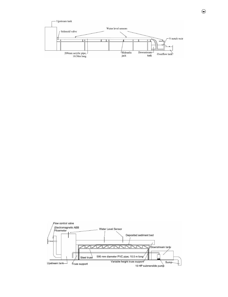
to a 200 mm solenoid valve, which controlled the inflow into
the setup from a 3.5 m
3
upstream tank. A downstream tank
with a V-Notch weir was used to measure the water discharge.
A real-time water level sensor was used to measure the water
height over the weir to calculate the water discharge rate using
the V-Notch equation. The calculated discharge was also
checked using an ABB- Electromagnetic flowmeter sensor
installed upstream of the pipe. Two additional real-time water
level sensors were installed along the pipe, aiming to measure
the stage hydrograph produced by the flushing waves.
Figure 1
shows the general scheme of the experimental setup.
The experimental data was collected as follows. Firstly, the
solenoid valve was fully opened, allowing a base flowrate ran-
ging from 0.002 l s
−1
to 0.414 l s
−1
. The opening of this valve
simulates the ‘dam break hydrograph’ produced during
a flushing operation in a real sewer pipe (e.g. using a Hydrass
or a Hydroself flushing gate). Secondly, a sediment bed with
near-uniform thickness and width was located at the bottom of
the pipe. At this point, the base flowrate helped the formation
of the deposited bed along a 3.3 m section. Thirdly, the sole-
noid valve was completely closed for storing a volume of water
between 0.10 m
3
and 0.31 m
3
in the upstream tank. Fourthly,
the solenoid valve was opened between 60% and 100% and
the opening time was set to 15 sec for all tests. When the first
discharged wave reached the sediment bed, the movement of
the bed was tracked over time. The sediment velocity (V
s
) was
calculated using the values of the time and deposited bed
displacement during the peak flow. The above procedure was
repeated for different accumulated upstream water volume
and percentage of the solenoid valve opening.
2.2. 595 mm pipe setup
The pipe was 10.5 m long and supported on a mechanical steel
truss, which allowed to modify the slope in a range between
0.04% and 3.44%. The base flow for the experiments, ranging
from 1.03 l s
−1
to 9.98 l s
−1
, was provided by a 40 BHP pump
that supplied water to a 30 m
3
upstream storage which was
directly connected to the pipe. For evaluating unsteady flow
conditions in this pipe, a second 10 BHP submersible pump was
located inside the downstream tank. This pump was directly
connected to the upstream tank and was controlled with
a variable frequency drive programmed before the experiment
to create a pulse with a maximum peak flow of 30 l s
−1
. Three
water level sensors were used to record water depths in the
experimental setup. Two of them were installed in the pipe to
collect the stage hydrograph, and one was installed in the
upstream tank. Full details of the experimental setup were
described in Montes et al. (
2020b
) and are shown in
Figure 2
.
For this setup, the data was collected as follows. Firstly, the
pipe slope was adjusted using the mechanical steel truss and
measured with a dumpy level. Secondly, the flow control valve
on the upstream tank was opened to supply a base flow to the
pipe. Thirdly, a deposited sediment bed with a near-uniform
width was prepared at the bottom of the pipe over a minimum
length of 1.5 m. At this point, to compare the flushing efficiency
under similar conditions, the maximum sediment bed velocity
was verified as 0.03 m s
−1
. If this condition was not fulfilled, the
pipe slope or the base flow were changed. Fourthly, the sub-
mersible pump, with its variable frequency drive, was activated
to simulate the ‘dam break hydrograph’, which is similar to those
produced by the flushing gates in real sewers. The water levels
were recorded each 0.025 s and the position of the sediment bed
Figure 1.
Experimental setup used to collect the unsteady flow data in the 209 mm acrylic pipe.
Figure 2.
Experimental setup used to collect the unsteady flow data in the 595 mm PVC pipe.
URBAN WATER JOURNAL
3
was tracked. The sediment velocity was calculated using the
same procedure followed on the acrylic setup.
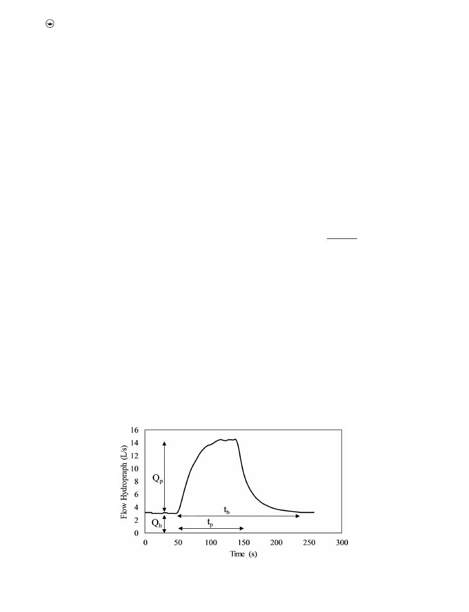
2.3. Experimental data collected
Using the experimental rig and approach described above,
a total of 57 and 64 experiments were carried out in the
209 mm acrylic pipe and 595 mm PVC pipe, respectively.
Several variables related to the pipe geometry, sediment prop-
erties, and flushing hydraulics, including the base time (t
b
),
peak time (t
p
), base flow (Q
b
), and peak flow (Q
p
) were recorded
in each experiment, as shown in
Figure 3
. The experimental
data collected in both acrylic and PVC pipes are presented in
Table 1
, where S
o
is the pipe slope, D the pipe diameter, Y the
water level in the pipe, R the hydraulic radius, d the mean
particle diameter, SG the specific gravity, y
s
the sediment thick-
ness, V
f
the water velocity, and V
s
the sediment velocity.
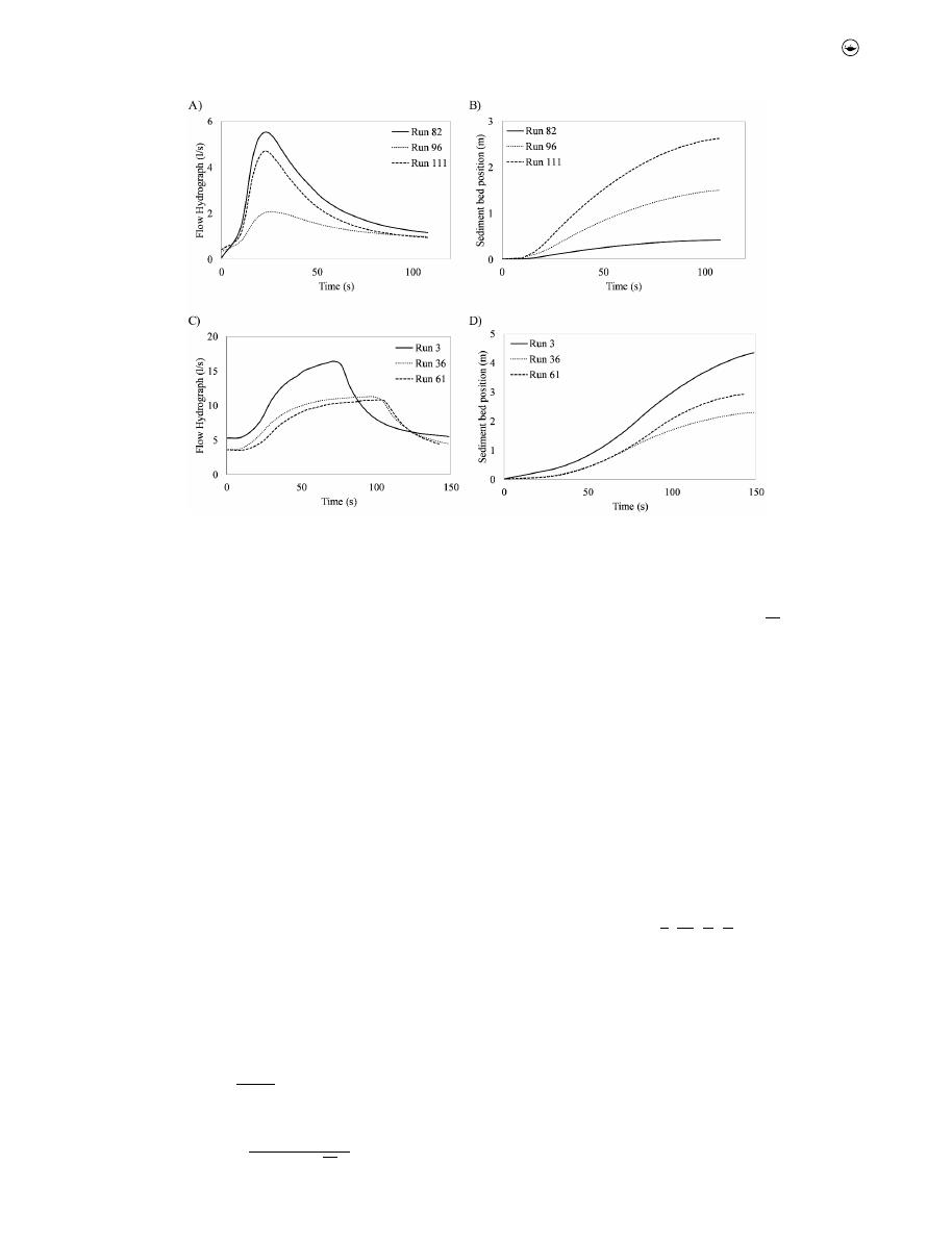
A flushing discharge hydrograph and a plot showing the
sediment bed position related with each run are presented in
Table 1
. The shape and magnitude of the hydrograph are
directly related to the sediment bed velocity, and consequently,
the sediment bed position. As an example, for six runs, the
variation in the sediment bed position and hydrograph char-
acteristics, in both acrylic and PVC pipe, are presented in
Figure 4
. Full details of each run shown in
Figure 4
are pre-
sented in
Table 1
.
Figure 4(a, b
) show the relation between the flushing dis-
charge hydrograph and the sediment bed position for tests
conducted on the acrylic pipe. As seen in these figures, particle
size is a more important variable in defining the sediment
position, compared to the peak flow in the hydrograph. Even
though the run 82 considers a higher peak flow (Q
p
= 5.55 l s
−1
),
the final position of the sediment bed (= 0.41 m) is lower than
the run 96 (= 2.62 m) when the peak flow is lower (Q
p
= 2.08 l
s
−1
). This occurs because the particle diameter is more relevant
compared to the peak flow.
Figure 4(c, d
) show the relation between the flushing dis-
charge hydrograph and the sediment bed position for tests in
595 mm setup. The relationship between the discharge hydro-
graph and the sediment bed position is proportional. For run
no. 36 and 61, the mean particle diameter was 2.60 mm, but the
pipe slope was 1.65% and 1.82%, respectively.
Figure 4(d
)
shows that maintaining the mean particle diameter constant
as the pipe slope increases, the final bed position increases.
3. Model development
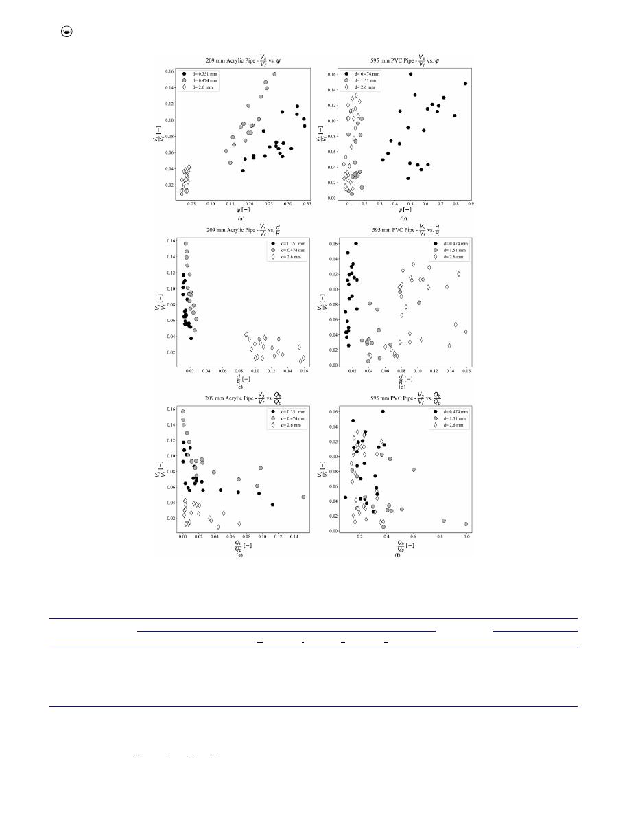
3.1. Graphical analysis
A graphical analysis was developed to visualize the relationships
between the variables collected in each experiment. The rela-
tionship between sediment velocity and flow velocity (V
s
=
V
f
) was
plotted against other dimensionless parameters, as shown in
Figure 5
. These dimensionless parameters have been previously
identified as relevant for predicting sediment transport in sewer
pipes in previous literature (Ab Ghani and Azamathulla
2011
;
Ebtehaj and Bonakdari
2016
; May et al.
1996
; Kuriqui, Koçileri,
and Ardiçlioğlu
2020
; Montes, Kapelan, and Saldarriaga
2021
).
Two of these parameters include the dimensionless grain size
(d=R) and the Shields parameter (ψ), defined in Equation (4):
ψ ¼
RS
o
SG
1
ð
Þ
d
(4)
Based on the results shown in
Figure 5
, the following observa-
tions can be made:
●
In general, higher values of the Shields parameter lead to
higher values of V
s
=
V
f
. This can be clearly seen in the acrylic
pipe (
Figure 5(a
)) because of the constant slope value
adopted in the experimental rig. Furthermore, high values
of S
o
and R lead to higher sediment velocities due to higher
critical shearing stress (i.e. the applied forces are higher
than the submerged weight of the particle). In contrast,
deposited materials with high density of particle diameters
result in lower sediment velocities.
●
The direct relationship between V
s
=
V
f
and the Shields
parameter coincides with the inversely proportional rela-
tionship between V
s
=
V
f
and d=R, shown in
Figure 5(c,d)
.
This is observed because the Shields parameter includes
the ratio R=d, as shown in Equation (4).
Figure 3.
Variable definition of the flushing discharge hydrograph.
4
C. MONTES ET AL.

Table 1.
Experimental data collected for studying flushing waves efficiency on sewer pipes.
Run no.
S
o
D
Y
R
d
SG
y
s
t
b
t
p
Q
b
Q
p
V
f
V
s
(%)
(mm)
(mm)
(mm)
(mm)
(-)
(mm)
(s)
(s)
(l s
−1
)
(l s
−1
)
(m s
−1
)
(m s
−1
)
1
0.805
595
70.35
41.96
0.47
2.66
10.14
154
59
5.27
25.48
1.02
0.07
2
0.805
595
57.43
34.62
0.47
2.66
8.26
141
57
5.45
16.76
0.89
0.05
3
0.805
595
53.61
31.34
0.47
2.66
10.53
131
57
5.45
16.49
0.82
0.04
4
1.186
595
57.82
36.46
0.47
2.66
2.49
121
59
4.89
20.53
1.20
0.05
5
1.229
595
54.70
31.17
0.47
2.66
12.55
115
55
4.81
15.97
0.99
0.03
6
1.229
595
61.66
36.67
0.47
2.66
9.91
120
55
5.07
20.27
1.14
0.04
7
1.229
595
50.94
31.92
0.47
2.66
3.90
183
58
1.03
11.10
1.09
0.05
8
1.229
595
67.63
39.54
0.47
2.66
12.15
124
57
5.03
24.47
1.19
0.05
9
1.229
595
62.04
37.24
1.51
2.66
8.97
39
33
9.98
12.06
1.16
0.02
10
1.525
595
42.69
22.71
1.51
2.66
13.54
117
58
5.17
11.84
0.87
0.02
11
2.034
595
37.55
19.29
1.51
2.66
13.28
111
59
4.92
11.54
0.89
0.09
12
2.331
595
35.95
19.45
1.51
2.66
10.96
182
57
3.99
10.93
0.97
0.10
13
0.763
595
67.43
38.31
1.51
2.66
14.87
113
56
4.42
11.71
0.90
0.00
14
0.763
595
70.23
39.60
1.51
2.66
15.99
126
69
9.13
22.46
0.92
0.03
15
0.763
595
81.75
47.82
1.51
2.66
13.12
135
63
9.40
31.43
1.07
0.04
16
1.123
595
58.13
34.59
1.51
2.66
9.55
118
60
9.23
17.93
1.04
0.03
17
1.123
595
64.66
37.76
1.51
2.66
11.97
118
57
9.37
22.36
1.10
0.04
18
1.186
595
57.59
29.85
1.51
2.66
19.13
149
79
3.59
20.04
0.92
0.07
19
1.186
595
52.88
28.98
1.51
2.66
14.70
149
88
3.95
16.45
0.91
0.04
20
1.186
595
64.30
36.57
1.51
2.66
14.31
195
93
3.51
24.52
1.09
0.09
21
0.847
595
69.70
40.25
1.51
2.66
13.64
185
55
3.72
20.71
0.99
0.03
22
0.847
595
51.24
28.32
1.51
2.66
13.83
104
8
7.28
7.33
0.76
0.01
23
1.589
595
32.25
14.83
1.51
2.66
14.35
118
82
4.36
7.24
0.65
0.05
24
0.847
595
63.16
36.41
2.60
2.64
12.98
120
76
4.71
12.53
0.92
0.01
25
0.847
595
66.11
36.30
2.60
2.64
17.48
156
86
4.10
16.57
0.90
0.01
26
0.847
595
72.84
43.20
2.60
2.64
10.93
161
83
4.13
20.88
1.06
0.03
27
0.847
595
105.64
61.10
2.60
2.64
15.39
167
65
4.11
24.98
1.34
0.02
28
1.059
595
62.36
34.80
2.60
2.64
15.48
143
75
4.22
11.91
0.99
0.01
29
1.059
595
54.15
28.78
2.60
2.64
16.77
154
83
4.02
16.63
0.85
0.03
30
1.186
595
59.13
33.26
2.60
2.64
14.30
143
67
3.69
19.77
1.01
0.03
31
1.186
595
67.08
38.56
2.60
2.64
13.76
148
74
3.57
23.71
1.14
0.02
32
1.483
595
39.34
18.73
2.60
2.64
16.36
176
88
3.45
10.96
0.73
0.02
33
1.483
595
46.74
24.88
2.60
2.64
14.66
136
80
3.52
15.45
0.91
0.03
34
1.483
595
53.25
28.81
2.60
2.64
15.54
186
72
3.39
19.73
1.01
0.04
35
1.483
595
59.57
32.28
2.60
2.64
16.95
184
79
3.42
23.61
1.10
0.07
36
1.653
595
38.51
16.34
2.60
2.64
19.13
134
82
3.75
11.36
0.69
0.03
37
1.653
595
46.08
23.02
2.60
2.64
17.21
141
84
3.76
15.96
0.90
0.09
38
1.653
595
52.56
28.02
2.60
2.64
16.18
146
70
3.71
20.08
1.04
0.12
39
1.653
595
59.13
33.13
2.60
2.64
14.58
147
64
3.64
23.79
1.19
0.12
40
1.568
595
38.73
18.76
0.47
2.66
15.60
135
87
3.64
11.58
0.76
0.06
41
1.568
595
46.16
24.41
0.47
2.66
14.80
142
81
3.73
15.96
0.92
0.08
42
1.568
595
53.90
29.62
0.47
2.66
14.77
146
87
3.66
20.35
1.07
0.09
43
1.568
595
59.10
34.08
0.47
2.66
12.39
151
81
3.75
24.25
1.20
0.13
44
1.822
595
37.55
18.70
0.47
2.66
14.29
140
87
4.06
11.92
0.82
0.09
45
1.822
595
45.29
22.96
0.47
2.66
16.33
148
88
4.00
16.48
0.95
0.13
46
1.822
595
51.59
29.70
0.47
2.66
11.33
152
81
3.95
20.87
1.17
0.14
47
2.034
595
35.08
19.49
0.47
2.66
9.71
121
84
3.97
10.64
0.92
0.15
48
2.034
595
42.85
24.99
0.47
2.66
9.05
161
89
3.26
14.75
1.11
0.13
49
2.034
595
50.35
30.68
0.47
2.66
6.79
7
78
3.56
20.07
1.32
0.14
50
2.034
595
54.22
33.47
0.47
2.66
5.64
178
60
3.56
23.79
1.42
0.21
51
2.246
595
34.90
21.54
0.47
2.66
4.68
127
75
4.36
11.38
1.09
0.13
52
2.246
595
42.64
25.31
0.47
2.66
7.95
159
77
3.78
15.90
1.19
0.15
53
2.246
595
35.17
17.28
2.60
2.64
13.82
131
78
4.07
11.19
0.86
0.10
54
2.246
595
42.78
22.75
2.60
2.64
13.58
142
88
3.62
15.55
1.06
0.14
55
2.246
595
47.24
27.46
2.60
2.64
9.96
146
85
3.62
19.82
1.24
0.17
56
2.246
595
52.77
31.74
2.60
2.64
8.10
142
79
3.72
23.74
1.40
0.18
57
2.076
595
36.93
19.14
2.60
2.64
12.77
136
85
3.90
11.87
0.90
0.09
58
2.076
595
43.16
24.38
2.60
2.64
10.84
11
77
3.69
16.02
1.09
0.12
59
2.076
595
50.20
28.50
2.60
2.64
11.99
153
92
3.67
20.34
1.21
0.14
60
2.076
595
54.70
32.31
2.60
2.64
9.85
154
79
3.79
24.16
1.35
0.14
61
1.822
595
36.34
17.74
2.60
2.64
14.46
123
84
3.54
10.84
0.79
0.04
62
1.822
595
43.56
25.20
2.60
2.64
9.63
162
85
3.20
15.12
1.05
0.12
63
1.822
595
50.97
30.34
2.60
2.64
8.79
171
78
3.18
19.05
1.21
0.09
64
1.822
595
56.21
32.54
2.60
2.64
11.66
168
87
3.25
23.71
1.25
0.11
65
0.644
209
34.99
20.17
2.60
2.64
5.60
101
18
0.08
3.80
0.55
0.02
66
0.644
209
49.27
27.29
2.60
2.64
8.22
101
16
0.01
6.60
0.68
0.02
67
0.644
209
51.63
27.99
2.60
2.64
9.89
101
14
0.02
6.84
0.68
0.02
68
0.644
209
28.15
16.32
2.60
2.64
4.98
101
20
0.14
1.99
0.48
0.01
69
0.644
209
30.78
16.70
2.60
2.64
7.96
101
19
0.11
2.45
0.47
0.00
70
0.644
209
40.49
23.10
2.60
2.64
6.26
101
17
0.08
4.73
0.61
0.02
71
0.644
209
53.26
29.33
2.60
2.64
8.49
101
15
0.02
7.37
0.71
0.03
72
0.644
209
35.58
20.28
2.60
2.64
6.26
101
20
0.12
3.62
0.55
0.01
73
0.644
209
40.61
23.32
2.60
2.64
5.82
101
18
0.06
4.58
0.62
0.02
(Continued)
URBAN WATER JOURNAL
5

●
Figure 5(e
) shows the inversely proportional relationship
between V
s
=
V
f
and the dimensionless parameter Q
b
=
Q
p
,
meaning that higher and steeper discharge hydrographs
(i.e. lower ratios Q
b
=
Q
p
) show higher V
s
=
V
f
values.
●
In general, based on what was previously mentioned,
higher values of S
o
and R and lower values of d, SG, and
Q
b
=
Q
p
lead to higher sediment velocities V
s
.
3.2. Evolutionary polynomial regression model
A new regression-based model was developed here to predict
the dimensionless ratio V
s
=
V
f
during flushing operation. The
new model includes the group of parameters identified in
previous studies (Ab Ghani and Azamathulla
2011
; Ebtehaj
and Bonakdari
2016
; May et al.
1996
; Montes, Kapelan, and
Saldarriaga
2021
) and the graphic analysis carried out for the
experimentally collected data, as shown in
Figure 5
.
Evolutionary polynomial regression (EPR) is a hybrid regres-
sion technique that combines numerical and symbolic regression
(Giustolisi and Savic
2006
,
2004
). In its original formulation, it
used single-objective genetic algorithms to explore the formula
space, and then it estimates the least-squares regression coeffi-
cients. This technique has proved to be effective when the
number of polynomial terms is not large (Giustolisi and Savic
2009
). To solve these issues, Giustolisi and Savic (Giustolisi and
Savic
2009
) introduced the EPR technique combined with
a Multi-Objective Genetic Algorithm (MOGA). This novel techni-
que maximises the model accuracy (i.e. minimises the sum of
squared errors) and minimises the number of polynomial coeffi-
cients, and therefore improves the exploration of the space of
Table 1.
(Continued).
Run no.
S
o
D
Y
R
d
SG
y
s
t
b
t
p
Q
b
Q
p
V
f
V
s
(%)
(mm)
(mm)
(mm)
(mm)
(-)
(mm)
(s)
(s)
(l s
−1
)
(l s
−1
)
(m s
−1
)
(m s
−1
)
74
0.644
209
45.95
25.29
2.60
2.64
8.76
101
17
0.03
5.42
0.64
0.01
75
0.644
209
52.17
28.92
2.60
2.64
7.96
101
16
0.03
7.22
0.71
0.03
76
0.644
209
29.87
16.87
2.60
2.64
6.26
101
21
0.11
2.06
0.48
0.01
77
0.644
209
33.61
19.44
2.60
2.64
5.39
101
19
0.10
2.75
0.54
0.01
78
0.644
209
44.28
24.82
2.60
2.64
7.45
101
18
0.02
5.17
0.64
0.02
79
0.644
209
47.12
26.13
2.60
2.64
8.22
101
18
0.01
5.90
0.66
0.02
80
0.644
209
38.03
21.54
2.60
2.64
6.72
101
19
0.08
3.80
0.58
0.01
81
0.644
209
41.49
23.59
2.60
2.64
6.49
101
18
0.05
4.59
0.62
0.02
82
0.644
209
43.13
23.90
2.60
2.64
8.22
101
17
0.04
5.55
0.61
0.01
83
0.644
209
44.99
24.43
2.60
2.64
9.60
101
16
0.02
6.11
0.62
0.02
84
0.644
209
38.93
21.05
2.60
2.64
9.31
101
18
0.04
4.51
0.55
0.01
85
0.644
209
47.10
25.93
2.60
2.64
8.76
101
17
0.02
5.83
0.65
0.01
86
0.644
209
38.30
22.59
0.47
2.66
3.91
101
17
0.10
4.36
0.62
0.06
87
0.644
209
51.25
29.60
0.47
2.66
3.68
101
16
0.00
7.36
0.76
0.11
88
0.644
209
52.44
29.99
0.47
2.66
4.65
101
15
0.01
7.64
0.75
0.10
89
0.644
209
29.07
17.09
0.47
2.66
4.40
101
19
0.21
2.22
0.50
0.03
90
0.644
209
33.05
19.59
0.47
2.66
3.91
101
17
0.19
2.65
0.56
0.04
91
0.644
209
41.19
24.21
0.47
2.66
3.86
101
18
0.04
4.99
0.65
0.08
92
0.644
209
56.85
32.46
0.47
2.66
3.51
101
15
0.00
8.02
0.81
0.13
93
0.644
209
39.63
23.20
0.47
2.66
4.40
101
17
0.07
4.08
0.62
0.05
94
0.644
209
43.42
25.52
0.47
2.66
3.46
101
17
0.08
4.99
0.68
0.06
95
0.644
209
47.40
27.47
0.47
2.66
4.21
101
16
0.04
5.56
0.71
0.07
96
0.644
209
30.86
18.45
0.47
2.66
3.46
101
19
0.32
2.08
0.54
0.03
97
0.644
209
32.77
19.21
0.47
2.66
4.59
101
20
0.11
2.80
0.54
0.04
98
0.644
209
42.21
24.97
0.47
2.66
3.03
101
19
0.41
4.22
0.67
0.06
99
0.644
209
37.41
21.71
0.47
2.66
5.18
101
19
0.09
3.79
0.59
0.05
100
0.644
209
41.66
24.19
0.47
2.66
4.86
101
17
0.07
4.63
0.64
0.05
101
0.644
209
43.34
25.14
0.47
2.66
4.78
101
18
0.06
5.71
0.66
0.06
102
0.644
209
48.65
28.13
0.47
2.66
4.21
101
16
0.03
6.67
0.72
0.09
103
0.644
209
36.32
21.27
0.35
2.65
4.59
101
18
0.06
4.24
0.58
0.05
104
0.644
209
51.00
29.01
0.35
2.65
5.60
101
15
0.01
6.81
0.73
0.08
105
0.644
209
50.99
29.11
0.35
2.65
5.18
101
15
0.01
6.90
0.73
0.09
106
0.644
209
28.62
16.45
0.35
2.65
5.39
101
18
0.23
2.00
0.48
0.02
107
0.644
209
32.66
18.92
0.35
2.65
5.26
101
17
0.19
2.67
0.53
0.03
108
0.644
209
42.79
24.72
0.35
2.65
5.18
101
16
0.07
4.80
0.65
0.04
109
0.644
209
54.41
30.76
0.35
2.65
5.60
101
17
0.00
7.36
0.76
0.07
110
0.644
209
37.13
21.55
0.35
2.65
5.18
101
18
0.10
3.75
0.59
0.03
111
0.644
209
41.56
24.21
0.35
2.65
4.59
101
17
0.08
4.71
0.64
0.05
112
0.644
209
45.08
25.81
0.35
2.65
5.73
101
17
0.07
5.47
0.67
0.05
113
0.644
209
54.08
30.60
0.35
2.65
5.60
101
15
0.03
7.31
0.76
0.08
114
0.644
209
29.46
16.96
0.35
2.65
5.39
101
20
0.19
2.02
0.49
0.03
115
0.644
209
33.04
18.92
0.35
2.65
5.90
101
19
0.13
2.74
0.53
0.03
116
0.644
209
44.81
25.64
0.35
2.65
5.82
101
17
0.04
5.18
0.66
0.04
117
0.644
209
48.43
27.71
0.35
2.65
5.39
101
17
0.02
5.88
0.70
0.05
118
0.644
209
39.31
22.65
0.35
2.65
5.60
101
18
0.09
3.92
0.60
0.04
119
0.644
209
41.99
24.16
0.35
2.65
5.60
101
17
0.08
4.59
0.63
0.04
120
0.644
209
43.59
25.04
0.35
2.65
5.60
101
18
0.04
5.64
0.65
0.04
121
0.644
209
44.65
25.62
0.35
2.65
5.60
101
17
0.06
6.12
0.66
0.07
6
C. MONTES ET AL.
symbolic formulas. EPR-MOGA considers some pseudo-
polynomial expressions such as (Giustolisi and Savic
2009
):
^
Y ¼ a
0
þ
X
m
j¼1
a
j
X
1
ð
Þ
ES j;1
ð
Þ
� . . . �
X
k
ð
Þ
ES j;k
ð
Þ
�
f
X
1
ð
Þ
ES j;kþ1
ð
Þ
�
�
� . . .
�
f
X
k
ð
Þ
ES j;2k
ð
Þ
�
�
(5)
where ^
Y is the vector of model predictions; ES and j the
matrix of candidate exponents and the inner function,
respectively, both selected by the user; m the number of
terms; a
0
the bias term; a
j
the adjustable parameters esti-
mated by linear least squares and X
j
the candidate expla-
natory variables. The inner function f defined by the user
can be logarithmic, exponential, tangent hyperbolic, or
secant hyperbolic, and must be selected according to the
physics of the problem studied. The EPR technique returns
a range of models showing the influence of different
explanatory factors by progressively adding these as
input variables to monomial formulas, starting from the
most important ones. For each EPR identified model, the
following performance indices are calculated: the Bayesian
Information Criterion (BIC) and the Coefficient of
Determination (R
2
), as shown in Equations (6) and (7),
respectively.
BIC ¼
1 þ d
log n
ð Þ
n
�
�
X
n
i¼1
Y
�
Y
ð
Þ
2
!
(6)
R
2
¼
1
P
n
i¼1
Y
�
Y
ð
Þ
2
P
n
i¼1
Y
�
Y
�
�
2
(7)
where Y
�
and Y are the observed and calculated data,
respectively, n is the number of data, d the number of
parameters included in the model and Y
�
the mean of
observed data. The Coefficient of Determination measures
the fraction of variance that can be explained. Note that
this coefficient varies between 0 and 1, where 1 denotes
a perfect match between observed and calculated data. The
Bayesian Information Criterion measures the trade-off
between accuracy and parsimony of the model. This mea-
sure penalises formulas with large number of parameters.
The model with the lowest BIC value is selected as optimal.
The new model was constructed to predict the dimension-
less relation V
s
=
V
f
, i.e., the vector of model predictions ^
Y is
defined as V
s
=
V
f
. The matrix of candidate exponents was
defined with values ranging from −2.50 to 2.50, considering
steps of 0.1, i.e. ES ¼
2:50; 1:40; . . . ; 1:40; 2:50
½
�
. The matrix
of candidate explanatory variables is defined as follows:
X
j
¼
ψ;
d
;
Q
b
Q
p
;
y
s
R
;
t
b
t
p
;
β
�
�
(8)
Using previous considerations, and randomly splitting the
experimental data collected on the 209 mm and 595 mm
pipes, for both training (75% of the data) and testing (25% of
the data) stages, the results shown in
Table 2
were obtained
using the EPR-MOGA strategy.
Table 2
shows the Pareto front (i.e. range of models) generated
by the EPR, together with the corresponding BIC and R
2
values. For
example, the best one input variable model includes only the
Shields parameter as an explanatory variable for predicting the
V
s
=
V
f
(V
s
=
V
f
¼
0:17ψ
0:5
). This is the least complex, i.e., most
parsimonious model hence, unsurprisingly, it has a rather low
prediction accuracy (BIC = −48.21 and R
2
= 0.38). In contrast, the
Figure 4.
Example of flow hydrographs and sediment bed position for several experiments shown in
Table 1
.
URBAN WATER JOURNAL
7
6-variable model includes all candidate explanatory factors
V
s
=
V
f
¼
2:48ψ
1:4 Q
b
Q
p
� �
0:3
d
R
�
0:9 y
s
R
�
0:1 t
b
t
p
� �
0:2
β
�
�
, resulting in
low parsimony model but with improved prediction accuracy
(BIC = −92.22 and R
2
= 0.64). Based on this, the model that
shows the best trade-off between accuracy and parsimony is the
model with three input variables. This model is shown in
Equation (9).
Figure 5.
Plots showing the relationships between the dimensionless velocity (V
s
=
V
f
) and other dimensionless variables in both acrylic and PVC pipe. Clustered results
by particle diameter.
Table 2.
Pareto solution provided by the EPR-MOGA strategy.
Terms of monomial formula
Performance Index
Number of inputs
Coefficient (a
j
)
ψ
Q
b
Q
p
d
R
y
s
R
t
b
t
p
β
BIC
R
2
1
0.17
0.50
-
-
-
-
-
−48.21
0.38
2
0.14
0.60
−0.10
-
-
-
-
−66.19
0.48
3
8.13
1.40
−0.30
0.90
-
-
-
−104.55
0.63
4
11.47
1.50
−0.30
1.00
0.10
-
-
−100.56
0.64
5
121.48
2.10
−0.20
1.60
0.80
0.10
-
−96.49
0.64
6
2.48
1.40
−0.30
0.90
0.10
−0.20
1.00
−92.22
0.64
8
C. MONTES ET AL.
V
s
V
f
¼
8:13
d
R
� �
0:90
RS
o
SG
1
ð
Þ
d
�
�
1:40
Q
b
Q
p
�
�
0:30
(9)
Or rearranging the above formula to simplify the d=R term:
V
s
V
f
¼
8:13
d
R
� �
0:50
S
o
SG
1
ð
Þ
�
�
1:40
Q
b
Q
p
�
�
0:30
(10)
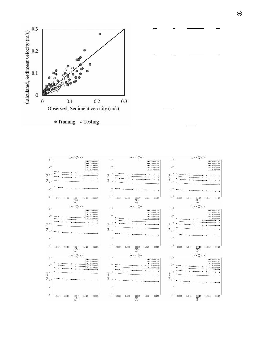
The obtained model was used to estimate the flushing effi-
ciency in larger pipes considering different flow conditions
and sediment characteristics. Further details are described in
the section below. The model’s accuracy can be seen in
Figure 6
for both training and testing datasets.
As it can be seen from the above equation and figure,
Equation (10) is consistent with the graphical analysis pre-
sented in
Figure 6
. Further, it can be seen from the model
obtained that
S
o
SG 1
ð
Þ
is the most important feature for predict-
ing the sediment velocity during the flushing cleaning opera-
tion – the more the pipe slope increases, the higher the particle
velocity is (note that the
S
o
SG 1
ð
Þ
parameter comes from the
Shields parameter). The Shields parameter shows the ratio
Figure 6.
EPR-MOGA model accuracy for both training and testing stage.
Figure 7.
Efficiency of flushing discharge vs particle diameter for several base and peak flow relations (0.25 < Q
b
=
Q
p
< 0.75) and pipe slope: a), b) and c) S
o
= 0.5%; d), e)
and f) S
o
= 1.0% and g), h) and i) S
o
= 1.5%.
URBAN WATER JOURNAL
9
between the hydrodynamic forces acting on the particles and
the resistance due to gravity. This parameter has been identi-
fied as one of the most relevant for predicting the incipient
motion in sewers (Delleur
2001
; Safari, Mohammadi, and Ab
Ghani
2018
; Wan Mohtar et al.
2018
). As mentioned above,
V
s
=
V
f
is inversely proportional to d=R, which is consistent with
the results shown by EPR-MOGA model.
4. Results and discussion
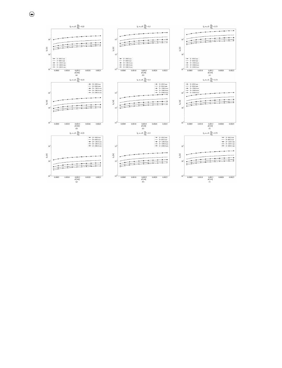
The new model shown in Equation (10) was used to generate
charts to estimate flushing efficiency as a function of the char-
acteristics of the discharged hydrograph, the pipe geometry
and the sediment properties. In this context, two flushing-
efficiency measures were defined as a function of the area of
deposited bed (A
s
) and the sediment velocity. The first measure,
Q
s
, is the volume of sediment removed by unit time (i.e. the
sediment flow rate = A
s
V
s
). The second measure, t
e
, is the
flushing time required to clean 1.0 m of the pipe (= 1=V
s
).
Figures 7 and 8
were constructed for several pipe diameters
using previous measures. To construct these figures, the less-
significant variables identified by the EPR-MOGA model (as
shown in
Table 2
) remained constant. The sediment thickness
was defined as y
s
=
D ¼ 1%, the specific gravity of the sediments
as 2.6, and the relation between the base and peak time of the
hydrograph as t
b
=
t
p
¼
5.0.
The following observations can be made from
Figures 7
and 8
:
●
Q
s
is inversely proportional to d and Q
b
=
Q
p
. In addition, Q
s
seems to be near-steady for particle diameters greater than
1.5 mm in pipes with diameters less than 800 mm. All above
for the same pipe slope and Q
b
=
Q
p
relation. Increasing the
pipe slope directly increase the sediment transport rate.
●
As the Q
b
=
Q
p
ratio increases, the sediment removal rate
decreases. For example, in
Figure 7(a
), when Q
b
=
Q
p
= 0.25
in a 1200 mm diameter pipe containing a deposited sedi-
ment bed with d = 1 mm, Q
s
= 0:5 � 10
−4
m
3
/s, while for
Q
b
=
Q
p
= 0.75 the Q
s
value changes to 0.2 � 10
−4
m
3
/s,
that is 60% less (as shown in
Figure 7(c
)).
●
Flushing discharges seem to be more efficient in larger
sewer pipes. The sediment transport rate can be five times
higher in 2000 mm diameter pipes, compared to
1200 mm diameter pipes.
●
Figure 8
shows a direct relationship between t
e
and d and
Q
b
=
Q
p
. Based on this, as d increases and Q
p
decreases, the
required flushing time to clean 1 meter of the pipe
increases. For example, in
Figure 8(d
) when Q
b
=
Q
p
=
0.25 in a 800 mm diameter pipe containing a deposited
sediment bed with d = 1.5 mm, t
e
= 20 sec, while for
Q
b
=
Q
p
= 0.75 the t
e
value changes to 45 sec, that is
125% more (as shown in
Figure 8(f
))
Figure 8.
Flushing time vs particle diameter for several base and peak flow relations (0.25 < Q
b
=
Q
p
< 0.75) and pipe slope: a), b) and c) S
o
= 0.5%; d), e) and f) S
o
= 1.0%
and g), h) and i) S
o
= 1.5%.
10
C. MONTES ET AL.

●
The flushing time decreases as the S
o
and D increase. That
is, flushing is a more efficient technique in large and steep
pipes.
4.1. Model comparison
To test the accuracy of the model shown in Equation (10), the
case study described in Laplace et al. (
2003
) was used. This case
study is located in Marseille, France, on a combined sewer net-
work. Specifically, this study considers an ovoid section of
1700 mm, 120 m long with a bottom slope of 0.03%. A near-
uniform deposited bed of 140 mm thickness was observed along
the entire length of the flume. The deposited bed was charac-
terised as coarser upstream (d = 8 mm) and finer downstream (d
= 0.6 mm). Full details are shown in Laplace et al. (
2003
).
Using a Hydrass-flushing gate located inside the section,
a series of flushes were conducted for testing the efficiency
on removing the deposited material. During each flush, a total
volume of 6.0 m
3
of water was discharged into the pipe. As
reported by Laplace et al. (
2003
), the mass of particles eroded
during the first flush was 6.3 kg, i.e., the removal rate was
1.08 kg of material per 1.0 m
3
of water (= 1.08 kg m
−3
).
Two existing procedures are compared with the new EPR-
MOGA model presented in Equation (10): the model proposed
by Bong, Lau, and Ab Ghani (
2013
) (i.e. Equation (3)) and the
design tables shown by Dettmar (
2007
). To compare the results,
several initial conditions are defined based on the case study
description, which are outlined as follows:
(1) Thickness of the deposited bed (y
s
) = 0.14 m
(2) Peak flow during flushing operation (Q
p
) = 100 l s
−1
(3) Specific gravity of the sediments (SG) = 2.60
(4) Mean particle diameter (d) = 0.6–8.0 mm
(5) Mass of material per meter of pipe = 54.22 kg m
−1
According to Bong, Lau, and Ab Ghani (
2013
), the number of
flushes required to move 1 m of deposited material can be
estimated by applying Equation (3). For this equation, the num-
ber of flushes is only a function of the thickness of the deposited
bed. As a result, 42 flushes (= 250.6 m
3
of water) can potentially
remove 54.22 kg of the deposited material (i.e. the removal rate is
0.21 kg m
−3
). Design tables proposed by Dettmar (
2007
) suggest
a flushing volume of 48 m
3
for a basic cleaning of the 150 m long
sewer (i.e. a full removing of the deposited material). No removal
rates are provided by Dettmar (
2007
).
Finally, using the new model proposed in this study, a range
of removal rates are obtained as a function of the mean particle
diameter. Potentially, a flushing volume of 10.18 m
3
can
remove 14.5 kg of deposited material with a mean particle
diameter of 0.6 mm (i.e. the removal rate is 0.40 kg m
−3
). By
changing the particle size of the deposited material to 8.3 mm,
the removal rate is 1.25 kg m
−3
.
As shown in
Table 3
, a direct comparison of the method
proposed by Dettmar (
2007
) and the results reported by
Laplace et al. (
2003
) is not possible. However, this method
seems to underestimate the real volume required to remove
the deposited bed. Relevant parameters such as the mean
particle diameter and the sewer hydraulics are not included in
this method. Due to the pipe slope in the case of study is almost
flat, obtaining minimum shear stress of 5.0 N m
−2
for cleaning
the pipe, according to Dettmar (
2007
), requires larger flows.
The model presented by Bong, Lau, and Ab Ghani (
2013
) is
a good approach for determining the number of flushes
required to move the deposited material. However, because
of the non-inclusion of relevant pipe hydraulics and sediment
parameters, the results are underestimated, compared to the
values reported by Laplace et al. (
2003
).
4.2. Model considerations
The new model presented here shows good prediction accu-
racy with the data reported by Laplace et al. (
2003
). This is
explained by the inclusion of relevant parameters for predicting
the removal rate during the flushing operation. The model also
shows good extrapolation capabilities under different sewer
diameters and a wide range of variations of the mean particle
diameter.
The Shields parameter was selected as the most important
one due to the highest value in the regression coefficient and
the Pareto solution provided by the EPR-MOGA strategy. This
was expected since this parameter determines the threshold
condition of sediment initiation motion. The sediment thick-
ness parameter is less important for defining the sediment
velocity during the flushing operation due to the low regres-
sion coefficient presented in
Table 2
. As a result, the model can
be used in both combined and storm sewers, where the sedi-
ment thickness ranges from 10 mm to 100 mm and 10 mm to
330 mm, respectively (Bong, Lau, and Ab Ghani
2016
).
The model includes the peak flow as an explanatory variable
for predicting sediment transport rate. Higher peak flow implies
a higher removal rate since higher shear stresses are generated
at the bottom of the pipe. The observed shear stress values
(ranging from 2.0 N/m
2
to 6.5 N/m
2
in the PVC pipe) are con-
sistent with those reported in the literature for the erosion and
transport of bed material (Dettmar
2007
; Campisano, Creaco,
Table 3.
Comparison of results for predicting the flushing efficiency in Laplace et al. (
2003
) case of study.
Reference
Removal
rate
[kg m
−3
]
Observations
Laplace et al. (
2003
)
0.93
Original case of Study reported in a trunk combined sewer in Marseille, France
Dettmar (
2007
)
-
Volume of water value reported to clean a pipe section of 150 m long. Relevant parameters as pipe slope and particle
diameter are not considered.
Bong, Lau, and Ab Ghani
(
2013
)
0.21
Good approximation. Experimental model (Equation (3)) obtained with a constant flume slope of 0.001.
EPR-MOGA Equation
(10)
0.4–1.25
Good performance for predicting the removal rate during flushing waves operation. Model consider relevant parameters as
the mean particle diameter and the pipe geometry.
URBAN WATER JOURNAL
11
and Modica
2008
; Yang et al.
2019
). However, since the model
only considers transport as bedload, some fine particles may be
eroded and transported in suspension (which has been identi-
fied as one of the major sources of pollution in CSO (Laplace
et al.
2003
; Saul et al.
2003
)), due to the high turbulence of the
flow. This is particularly important in well-graded materials
where wide ranges of mean particle sizes are present.
Even though the new model was developed considering
a wide range of variations in input variables, some limitations
exist. The granular material used in the experiments cannot
represent the cohesive properties of sediments found in real
sewer systems. As a result, an increased bed resistance to
erosion can be seen in practice (Campisano et al.
2019
). In
addition, the lowest pipe slope value considered during the
tests was 0.644%, which is higher than the minimum self-
cleansing value recommended in several industry design
codes and water utilities design manuals (e.g. Health Research
Inc (
2004
), as quoted by Montes et al. (
2019
)).
5. Conclusions
This study proposes a simple model to predict the sediment
transport rate in practice based on data collected from a set of
121 lab experiments conducted on a 209 mm diameter acrylic
pipe and 595 mm diameter PVC pipe. The data collected this
way were processed using the EPR-MOGA modelling techni-
que. A new model for predicting the sediment velocity during
flushing operation was developed and used for constructing
design charts. Based on the results obtained, the following
conclusions are made:
(1) The new model developed and presented here can pre-
dict the sediment transport rate during flushing dis-
charges accurately in practice. This model includes the
group of parameters that most affect the flushing effi-
ciency in sewer pipes.
(2) The sediment transport rate is principally affected by
four parameters: pipe slope, pipe diameter, particle dia-
meter and discharged peak flow. In pipes with large
diameters and slopes, the flushing is more effective.
This is because of the high regression exponents for
both
S
o
SG 1
ð
Þ
and d=R variables obtained in the EPR-
MOGA model presented here. The sediment transport
is not significantly affected by the value of the deposited
sediment thickness.
(3) The new model proposed outperforms the simplified
models and methods reported in the literature in terms
of removal sediment rate prediction. This is seen by the
better prediction accuracy shown when compared to
the case study reported by Laplace et al. (
2003
).
(4) Existing models such as Bong, Lau, and Ab Ghani (
2013
)
and Dettmar (
2007
) for predicting sediment transport
tend to underestimate the total volume of water
required to clean a deposited sediment bed. The EPR-
MOGA model is more accurate in predicting the sedi-
ment transport rate as this model includes parameters
affecting the flushing efficiency, such as flushing hydrau-
lics, pipe geometry and sediment properties.
Based on the conclusions mentioned above, the new flush-
ing model can be useful for designing flushing schemes during
the operational stage of existing sewer pipes in engineering
practice. Further research is recommended to test the model
proposed in real sewer pipes under different sediment (i.e.
cohesive materials) and hydraulic conditions.
Acknowledgement
The authors would like to thank Professor Orazio Giustolisi who developed
and made available for free the EPR-MOGA XL software used in this
research.
Disclosure statement
No potential conflict of interest was reported by the author(s).
ORCID
Carlos Montes
http://orcid.org/0000-0003-0758-4697
Sergio Vanegas
http://orcid.org/0000-0001-5786-9450
Zoran Kapelan
http://orcid.org/0000-0002-0934-4470
Luigi Berardi
http://orcid.org/0000-0002-6252-2467
Juan Saldarriaga
http://orcid.org/0000-0003-1265-2949
References
Ab Ghani, A., and H. Azamathulla.
2011
. “Gene-Expression Programming for
Sediment Transport in Sewer Pipe Systems.” Journal of Pipeline Systems
Engineering and Practice 2 (3): 102–106. doi:
10.1061/(ASCE)PS.1949-
1204.0000076
.
Ashley, R., J. Bertrand-Krajewski, T. Hvitved-Jacobsen, and M. Verbanck.
2004
. Solids in Sewers: Characteristics, Effects and Control of Sewer Solids
and Associated Pollutants. London: IWA Publishing. doi:
10.2166/
9781780402727
.
ASTM D854-14.
2014
. Standard Test Methods for Specific Gravity of Soil
Solids by Water Pycnometer. West Conshohocken, PA: ASTM
International.
Bajirao, T., P. Kumar, M. Kumar, A. Elbeltagi, and A. Kuriqi.
2021
. “Superiority
of Hybrid Soft Computing Models in Daily Suspended Sediment
Estimation in Highly Dynamic Rivers.” Sustainability 13 (2): 542.
doi:
10.3390/su13020542
.
Bertrand-Krajewski, J., J. Bardin, C. Gibello, and D. Laplace.
2003
. “Hydraulics
of a Sewer Flushing Gate.” Water Science and Technology 47 (4): 129–136.
doi:
10.2166/wst.2003.0237
.
Bong, C., T. Lau, and A. Ab Ghani.
2013
. “Hydraulics Characteristics of
Tipping Sediment Flushing Gate.” Water Science and Technology
68 (11): 2397–2406. doi:
10.2166/wst.2013.498
.
Bong, C., T. Lau, and A. Ab Ghani.
2016
. “Potential of Tipping Flush
Gate for Sedimentation Management in Open Stormwater Sewer.”
Urban
Water
Journal
13
(5):
486–498.
doi:
10.1080/
1573062X.2014.994002
.
Campisano, A., and C. Modica.
2003
. “Flow Velocities and Shear Stresses
during Flushing Operations in Sewer Collectors.” Water Science and
Technology 47 (4): 123–128. doi:
10.2166/wst.2003.0236
.
Campisano, A., C. Modica, E. Creaco, and G. Shahsavari.
2019
. “A Model for
Non-uniform Sediment Transport Induced by Flushing in Sewer
Channels.”
Water
Research
163:
114903.
doi:
10.1016/j.
watres.2019.114903
.
Campisano, A., E. Creaco, and C. Modica.
2004
. “Experimental and
Numerical Analysis of the Scouring Effects of Flushing Waves on
Sediment Deposits.” Journal of Hydrology 299 (3–4): 324–334.
doi:
10.1016/j.jhydrol.2004.08.009
.
Campisano, A., E. Creaco, and C. Modica.
2006
. “Experimental Analysis of the
Hydrass Flushing Gate and Laboratory Validation of Flush Propagation
12
C. MONTES ET AL.

Modelling.” Water Science and Technology 54 (6–7): 101–108.
doi:
10.2166/wst.2006.608
.
Campisano, A., E. Creaco, and C. Modica.
2007
. “Dimensionless Approach for
the Design of Flushing Gates in Sewer Channels.” Journal of Hydraulic
Engineering 133 (8): 964–972. doi:
10.1061/(ASCE)0733-9429(2007)
133:8(964)
.
Campisano, A., E. Creaco, and C. Modica.
2008
. “Laboratory Investigation on
the Effects of Flushes on Cohesive Sediment Beds.” Urban Water Journal
5 (1): 3–14. doi:
10.1080/15730620701726259
.
Caviedes-Voullième, D., M. Morales-Hernández, C. Juez, A. Lacasta, and
P. García-Navarro.
2017
. “Two-dimensional Numerical Simulation of
Bed-load Transport of a Finite-depth Sediment Layer: Applications to
Channel Flushing.” Journal of Hydraulic Engineering 143 (9): 04017034.
doi:
10.1061/(ASCE)HY.1943-7900.0001337
.
Chebbo, G., D. Laplace, A. Bachoc, Y. Sanchez, and B. Le Guennec.
1996
.
“Technical Solutions Envisaged in Managing Solids in Combined Sewer
Networks.” Water Science and Technology 33 (9): 237–244. doi:
10.1016/
0273-1223(96)00392-7
.
Creaco, E., and J. Bertrand-Krajewski.
2009
. “Numerical Simulation of
Flushing Effect on Sewer Sediments and Comparison of Four Sediment
Transport Formulas.” Journal of Hydraulic Research 47 (2): 195–202.
doi:
10.3826/jhr.2009.3363
.
De Sutter, R., M. Huygens, and R. Verhoeven.
1999
. “Unsteady Flow
Sediment Transport in a Sewer Model.” Water Science and Technology
39 (9): 121–128. doi:
10.1016/S0273-1223(99)00224-3
.
Delleur, J.
2001
. “New Results and Research Needs on Sediment Movement
in Urban Drainage.” Journal of Water Resources Planning and
Management 127 (3): 186–193. doi:
10.1061/(ASCE)0733-9496(2001)
127:3(186)
.
Dettmar, J.
2005
. “Beitrag zur Verbesserung der Reinigung von
Abwasserkanälen.” PhD diss., RWTH Aachen University.
Dettmar, J.
2007
. “A New Planning Procedure for Sewer Flushing.” Paper
presented at the NOVATECH 2007 – Sixth International Conference on
Sustainable Techniques and Strategies in Urban Water Management,
Lyon, June 25–28.
Dettmar, J., B. Rietsch, and U. Lorenz.
2002
. “Performance and
Operation of Flushing Devices - Results of a Field and Laboratory
Study.” Global Solutions for Urban Drainage: Proceedings of the Ninth
International Conference on Urban Drainage 1–10. doi:
10.1061/40644-
(2002)291
.
Ebtehaj, I., and H. Bonakdari.
2016
. “Bed Load Sediment Transport in Sewers
at Limit of Deposition.” Scientia Iranica 23 (3): 907–917. doi:
10.24200/
sci.2016.2169
.
Ebtehaj, I., H. Bonakdari, S. Shamshirband, Z. Ismail, and R. Hashim.
2017
.
“New Approach to Estimate Velocity at Limit of Deposition in Storm
Sewers Using Vector Machine Coupled with Firefly Algorithm.” Journal of
Pipeline Systems Engineering and Practice 8 (2): 04016018. doi:
10.1061/
(ASCE)PS.1949-1204.0000252
.
Fan, C.
2004
. Sewer Sediment and Control A Management Practices Reference
Guide, EPA/600/R-04/059. Washington, DC: U.S. Environmental Protection
Agency.
Fan, C., R. Field, W. Pisano, J. Barsanti, J. Joyce, and H. Sorenson.
2001
.
“Sewer and Tank Flushing for Sediment, Corrosion, and Pollution
Control.” Journal of Water Resources Planning and Management 127 (3):
194–201. doi:
10.1061/(ASCE)0733-9496(2001)127:3(194)
.
Giustolisi, O., and D. Savic.
2004
. “A Novel Genetic Programming Strategy:
Evolutionary Polynomial Regression.” Proceedings of the 6th International
Conference
on
Hydroinformatics
787–794.
doi:
10.1142/
9789812702838_0097
.
Giustolisi, O., and D. Savic.
2006
. “A Symbolic Data-driven Technique Based
on Evolutionary Polynomial Regression.” Journal of Hydroinformatics
8 (4): 207–222. doi:
10.2166/hydro.2006.020
.
Giustolisi, O., and D. Savic.
2009
. “Advances in Data-driven Analyses and
Modelling Using EPR-MOGA.” Journal of Hydroinformatics 11 (3–4):
225–236. doi:
10.2166/hydro.2009.017
.
Guo, Q., C. Fan, R. Raghaven, and R. Field.
2004
. “Gate and Vacuum Flushing
of Sewer Sediment: Laboratory Testing.” Journal of Hydraulic Engineering
130 (5): 463–466. doi:
10.1061/(ASCE)0733-9429(2004)130:5(463)
.
Health Research Inc.
2004
. “Recommended Standards for Wastewater
Facilities.” A Report of the Wastewater Committee 12224 (518): 1–102.
Khosravi, K., J. Cooper, P. Daggupati, B. Thai Pham, and D. Tien Bui.
2020
.
“Bedload Transport Rate Prediction: Application of Novel Hybrid Data
Mining Techniques.” Journal of Hydrology 585: 124774. doi:
10.1016/j.
jhydrol.2020.124774
.
Kuriqui, A., G. Koçileri, and M. Ardiçlioğlu.
2020
. “Potential of Meyer-Peter
and Müller Approach for Estimation of Bed-load Sediment Transport
under Different Hydraulic Regimes.” Modeling Earth Systems and
Environment 6: 129–137. doi:
10.1007/s40808-019-00665-0
.
Lainé, S., L. Phan, D. Malabat, and B. Duffros.
1998
. “Flush Cleaning of
Sewer Using the Hydras-Valve.” Paper presented at the 4th
International Conference on Urban Drainage Modelling, London,
September 21–24.
Laplace, D., C. Oms, M. Ahyerre, G. Chebbo, J. Lemasson, and L. Felouzis.
2003
. “Removal of the Organic Surface Layer in Combined Sewer
Sediment Using a Flushing Gate.” Water Science and Technology 47 (4):
19–26. doi:
10.2166/wst.2003.0211
.
May, R., J. Ackers, D. Butler, and S. John.
1996
. “Development of Design
Methodology for Self-cleansing Sewers.” Water Science and Technology
33 (9): 195–205. doi:
10.1016/0273-1223(96)00387-3
.
Montes, C., J. Bohorquez, S. Borda, and J. Saldarriaga.
2019
. “Impact of
Self-Cleansing Criteria Choice on the Optimal Design of Sewer
Networks in South America.” Water (Switzerland) 11 (6): 1148.
doi:
10.3390/w11061148
.
Montes, C., L. Berardi, Z. Kapelan, and J. Saldarriaga.
2020a
. “Predicting
Bedload Sediment Transport of Non-cohesive Material in Sewer Pipes
Using Evolutionary Polynomial Regression – Multi-objective Genetic
Algorithm Strategy.” Urban Water Journal 17 (2): 154–162. doi:
10.1080/
1573062X.2020.1748210
.
Montes, C., S. Vanegas, Z. Kapelan, L. Berardi, and J. Saldarriaga.
2020b
.
“Non-deposition Self-cleansing Models for Large Sewer Pipes.” Water
Science and Technology 81 (3): 606–621. doi:
10.2166/wst.2020.154
.
Montes, C., Z. Kapelan, and J. Saldarriaga.
2021
. “Predicting Non-deposition
Sediment Transport in Sewer Pipes Using Random Forest.” Water
Research 189: 116639. doi:
10.1016/j.watres.2020.116639
.
NEIWPCC.
2003
. Optimizing Operation, Maintenance, and Rehabilitation of
Sanitary Sewer Collection Systems. Lowell, MA: New England Interstate
Water Pollution Control Commission.
Ristenpart, E.
1998
. “Solids Transport by Flushing of Combined Sewers.”
Water Science and Technology 37 (1): 171–178. doi:
10.1016/S0273-
1223(97)00767-1
.
Rodríguez, J., N. McIntyre, M. Díaz-Granados, and Č. Maksimović.
2012
.
“A Database and Model to Support Proactive Management of
Sediment-related Sewer Blockages.” Water Research 46 (15):
4571–4586. doi:
10.1016/j.watres.2012.06.037
.
Saegrov, S.
2006
. Computer Aided Rehabilitation of Sewer and Storm Water
Networks – CARE-S. IWA Publishing. doi:
10.2166/9781780402390
.
Safari, M.
2020
. “Hybridization of Multivariate Adaptive Regression Splines
and Random Forest Models with an Empirical Equation for Sediment
Deposition Prediction in Open Channel Flow.” Journal of Hydrology 590:
125392. doi:
10.1016/j.jhydrol.2020.125392
.
Safari, M., M. Mohammadi, and A. Ab Ghani.
2018
. “Experimental Studies of
Self-cleansing Drainage System Design: A Review.” Journal of Pipeline
Systems Engineering and Practice 9 (4): 04018017. doi:
10.1061/(ASCE)
PS.1949-1204.0000335
.
Sakakibara, T.
1996
. “Sediments Flushing Experiment in a Trunk Sewer.”
Water Science and Technology 33 (9): 229–235. doi:
10.1016/0273-
1223(96)00391-5
.
Saul, A., P. Skipworth, S. Tait, and P. Rushforth.
2003
. “Movement of Total
Suspended Solids in Combined Sewers.” Journal of Hydraulic Engineering
129 (4): 298–307. doi:
10.1061/(ASCE)0733-9429(2003)129:4(298)
.
Schaffner, J., and J. Steinhardt
2006
. “Numerical Investigation of the
Self-acting Flushing System HydroFlush GS in Frankenberg/Germany.”
Paper presented at the 2th Conference on Sewer Operation and
Maintenance, Vienna, October.
Shahsavari, G., G. Arnaud-Fassetta, and A. Campisano.
2017
. “A Field
Experiment to Evaluate the Cleaning Performance of Sewer Flushing
URBAN WATER JOURNAL
13

on Non-uniform Sediment Deposits.” Water Research 118: 59–69.
doi:
10.1016/j.watres.2017.04.026
.
Shirazi, R., A. Campisano, C. Modica, and P. Willems.
2014
. “Modelling the
Erosive Effects of Sewer Flushing Using Different Sediment Transport
Formulae.” Water Science and Technology 69 (6): 1198–1204. doi:
10.2166/
wst.2013.810
.
Wan Mohtar, W., H. Afan, A. El-Shafie, C. Bong, and A. Ab Ghani.
2018
.
“Influence of Bed Deposit in the Prediction of Incipient Sediment Motion
in Sewers Using Artificial Neural Networks.” Urban Water Journal 15 (4):
296–302. doi:
10.1080/1573062X.2018.1455880
.
Yang, H., D. Zhu, Y. Zhang, and Y. Zhou.
2019
. “Numerical Investigation on
Bottom Shear Stress Induced by Flushing Gate for Sewer Cleaning.”
Water Science and Technology 80 (2): 290–299. doi:
10.2166/wst.2019.269
.
Yu, C., and J. Duan.
2014
. “Two-Dimensional Finite Volume Model for
Sediment Transport in Unsteady Flow.” World Environmental and Water
Resources Congress 2014: 1432–1441. doi:
10.1061/9780784413548.144
.
14
C. MONTES ET AL.
