
water
Article
Impact of Self-Cleansing Criteria Choice on the
Optimal Design of Sewer Networks in South America
Carlos Montes
1
, Zoran Kapelan
2
and Juan Saldarriaga
3,
*
1
Water Supply and Sewer Systems Research Center (CIACUA), Universidad de los Andes,
Bogotá 111711, Colombia; cd.montes1256@uniandes.edu.co
2
Faculty of Civil Engineering and Geosciences, Delft University of Technology, 2600 AA Delft, The Netherlands;
Z.Kapelan@tudelft.nl
3
Department of Civil and Environmental Engineering, Universidad de los Andes, Bogotá 111711, Colombia
*
Correspondence: jsaldarr@uniandes.edu.co; Tel.:
+57-1-339-49-49 (ext. 3282)
Received: 20 February 2019; Accepted: 10 April 2019; Published: 31 May 2019
Abstract:
This paper aims to analyze di
fferent sediment self-cleansing criteria and to find out what
the corresponding implications are on the optimal design of sewer systems. A methodology based
on enumeration is used to find the sewer network design that minimizes the costs of construction
while fulfilling a number of design criteria including self-cleansing constraints. Three stormwater
and wastewater sewer networks are used for the analyses. The results indicate that in cases where
the terrain slopes and design flow rates are higher, the self-cleansing restrictions are irrelevant to
the optimal design. However, when the terrain slopes and the design flow rates are lower, these
restrictions a
ffect the final design. Using the results obtained, a graph is constructed showing the
limit at which self-cleansing restrictions become a constraining parameter in optimal design for sewer
networks. It is expected that this graph will be useful for the design of future sewer networks in
low-income areas, where the design of traditional, gravity-based sewer systems is essential.
Keywords:
self-cleansing sewer systems;
self-cleansing criteria;
sewer system optimal
design; sedimentation
1. Introduction
Sewer systems can be defined as an infrastructure used to collect and transport stormwater
and wastewater produced in urban areas. Traditionally, these systems have been designed without
considering optimization criteria, which has resulted in high construction costs and overdesigned
sewer networks. Recently, several techniques have been proposed to reduce construction costs.
These techniques include typical recommendations and constraints proposed in several water utilities
design manuals. Some of these constraints include minimum velocities or minimum shear stress values
to guarantee self-cleansing conditions in sewer systems.
The traditional design of sewer networks has been considered to be a single-objective strategy, i.e.,
without including construction costs. Recently, several authors have used multi-objective strategies,
which consider an optimal design of sewer pipes while a cost function equation is being minimized.
Techniques such as dynamic programming [
1
,
2
], nonlinear programming [
3
], random search [
4
],
LP-based heuristic approach [
5
], genetic algorithms [
6
–
10
], automated algorithm combining hydraulic
and hydrological simulation [
11
], and DP-based optimization engine [
12
], amongst other approaches,
have been used for the optimal design of sewer systems. Each of these approaches has been used in
several benchmark sewer networks, e.g., Mays and Wenzel [
13
] stormwater sewer network, taking into
account di
fferent cost function equations and design constraints.
Water 2019, 11, 1148; doi:10.3390
/w11061148
www.mdpi.com
/journal/water

Water 2019, 11, 1148
2 of 12
Part of the design constraints included in water utilities design manuals relate to self-cleansing
capacity. In this context, the concept of self-cleansing sewer systems has been introduced in sanitary
engineering practices. These systems must guarantee that transported particles do not deposit at the
bottom of the pipes, avoiding problems such as changes in the pipe cross-section or variations in
the water velocity profiles [
14
]. Some phenomena associated with these problems include blockages,
overcharges, water quality, and flooding.
In order to prevent problems such as the previously stated ones, several minimum velocities,
and minimum shear stress values have been proposed in the design manuals of di
fferent countries.
Usually, self-cleansing criteria depends on the type of sewer, i.e., stormwater, wastewater or combined
sewer system, and sometimes on the pipe’s diameter, e.g., Germany [
15
]. On the basis of this criteria,
Table
1
summarizes traditional values of self-cleansing criteria, obtained from the previous studies
of Vongvisessomjai et al. [
16
] and complemented with self-cleansing criteria collected in the United
States, Europe, and Latin American water utilities [
17
]. These values have traditionally been used in
the design of small sewer networks [
16
] and are widely employed today.
Table 1.
Minimum velocity and shear stress values.
Criterion No.
Source
Country
Sewer Type
v
min
[m
/s]
τ
min
[Pa]
(1)
Lysne [
18
]
USA
All
-
2.0–4.0
(2)
ASCE [
19
]
USA
WW
0.6
-
SW
0.9
-
(3)
Yao [
20
]
USA
SW
-
3.0–4.0
WW
-
1.0–2.0
(4)
Minister of Interior [
21
]
France
WW
0.3
-
C
0.6
-
(5)
British Standard BS 8001 [
22
]
UK
SW
0.75
-
C
1
-
(6)
Ecuadorian Normalization Institute (Instituto Ecuatoriano de
Normalización) [
23
]
Ecuador
WW
0.45
-
SW
0.9
-
(7)
European Standard EN 752-4 [
24
]
Europe
All
0.7
-
(8)
ATV-DVWK-Regelwerk [
15
]
Germany
All
Depends on pipe diameter
-
(9)
Great Lakes [
25
]
USA
WW
0.6
-
(10)
National Water Commission (Comisión Nacional del Agua) [
26
]
Mexico
SW
0.6
-
WW
0.3
-
(11)
Bolivian Institute for Standarization and Quality (Instituto
Boliviano de Normalización y Calidad) [
27
]
Bolivia
WW
-
1
SW and C
-
1.5
(12)
Medellin Public Enterprises (Empresas Públicas de Medellín) [
28
]
Colombia
WW
0.45
1.5
SW and C
0.75
3
(13)
Colombia. Ministry of Housing, City and Territory (Colombia.
Ministerio de Vivienda, Ciudad y Territorio) [
29
]
Colombia
WW
0.45
1.5
SW and C
0.75
3
Note: WW, wastewater; SW, stormwater; C, combined; All, all sewers.
The self-cleansing criteria, shown above, are commonly used to avoid the problems aforementioned.
In addition, the criteria shown in Table
1
cover the range of variation found in water utilities design
manuals. These values vary in di
fferent manuals and regions because of different climate conditions,
lifestyles, and cultures of people. These variations in self-cleansing criteria have usually been discussed
by water utilities, since there is no agreement that establishes a definitive or permanent self-cleansing
criterion. On the basis of previous concepts, this paper aims to evaluate the impact of di
fferent
self-cleansing criteria, as shown in Table
1
, on the optimal design of sewer networks. This evaluation is
important, especially in low-income areas of South America, where the design of gravity-based sewer
systems is essential, and the implementation of non-traditional systems, i.e., systems that consider
pump infrastructure, is usually not possible. In this context, a preliminary assessment of the impact
of self-cleansing criteria, especially in flat areas with low population density, on the design of future
sewer networks is essential to the evaluation of the feasibility of implementing a sewer system. In areas
where this is not possible, other solutions should be implemented, such as condominial sewer systems
or septic tanks, among others.
The remainder of the paper is organized as follows: Section
2
presents the methodology used
for the optimal design of sewer systems, the cost function, the hydraulic design constraints, and case
studies. Section
3
contains the solution of each network and the preliminary results. Section
4
presents a
sensitivity analysis which is performed to establish the limits of the terrain slope and design flow where
self-cleaning criteria a
ffect the final optimized network design. Section
5
outlines the conclusions.

Water 2019, 11, 1148
3 of 12
2. Methodology
2.1. Optimal Sewer Network Design
2.1.1. Design Cost
The sewer design methodology used in this study is described by Duque et al. [
12
]. It is a
three-step approach, based on graph modeling and shortest path algorithm, which is solved using
the Bellman–Ford algorithm [
30
]. In this approach, an exhaustive search is used to find the best
combination of slope and diameter for each pipe in a sewer network. The best combination chosen
guarantees a minimum total cost of the network, represented by Equation (1), fulfilling the design
constraints shown in Table
2
.
Table 2.
Hydraulic design constraints modified from Duque et al. [
12
].
Design Constraint
Threshold Value
Minimum diameter
200 mm
Maximum filling ratio
0.85
Minimum self-cleansing velocity
0.6–0.9 m
/s
Minimum shear stress
2.0–4.0 Pa
Maximum velocity
5.0 m
/s
Minimum depth below ground level
1.2 m
Maximum depth below ground level
5.0 m
In this methodology, each graph is considered as a combination of nodes (manholes) and arcs
(pipes), representing a single sewer design with a specific cost and a combination of diameter and slope
of each pipe. In addition, each manhole is represented by a subset of elevation and diameter. On the
basis of this information, each pipe in the network is created by joining two consecutive manholes
with a specific upstream and downstream elevation, i.e., with a specific slope and diameter. The subset
of diameters depends on the commercially available diameters.
The methodology has been tested for several sizes of networks, varying the number of pipes from
5 to 20. According to Duque et al. [
12
], the number of pipes and the terrain topography (steep or flat
terrain) a
ffect the computational time. As an example, the computational time required to solve a
network with five pipes located in a flat topography is close to 45 s; in contrast, the computational time
required to solve a network with 20 pipes located in a steep topography is about 190 s. As previously
mentioned, this methodology allows for the design of sewer networks in a short time. The full details
of this methodology are outlined by Duque et al. [
12
].
The total cost function used for the analyses is a regression-based cost model, developed using data
from di
fferent sources such as the Ministry of Environment (Colombia), the Housing and Territorial
Development (Ministerio de Ambiente, Vivienda y Desarrollo Territorial, in Spanish), the Financial
Fund for Development Projects (Fondo Financiero de Proyectos de Desarrollo FONADE, in Spanish),
and from sewage and water utilities. Equation (1) presents the cost function where C represents the
total cost (USD), D is the pipe diameter (mm), l is the pipe length (m) and V is the excavated volume
(m
3
), as defined in Equation (2).
C
=
1.32
2, 800
9579 D
0.57
l
+
1163 V
1.31
(1)
V
=
D
+
2e
+
0.15
+
H
+
H
0
2
!
×
(
2B
+
2e
+
D
)
×
l cos
tan
−1
S
o
(2)
where e is the wall thickness of the pipe (m); H and H
0
are the excavation limits above the top of the
pipe in the upstream and downstream of the pipe (m), respectively; B is the width of trench (m); and S
o
is the pipe slope (m
/m).
Water 2019, 11, 1148
4 of 12
The cost equation shown above is deemed appropriate for the work done here with this
methodology. This equation is useful for analyses, especially in South America, because it was
developed using information available in the region. However, the methodology presented in this
paper is generic in the sense that it allows alternative cost model(s) equations to be used, e.g.,
Maurer et al. [
31
], Moeini and Afshar [
32
] and Marchionni et al. [
33
], amongst others.
2.1.2. Design Constraints
Several design constraints are considered to ensure proper operation of sewer systems.
These constraints are usually recommended by the technical standards of each water utility. This study
takes the following restrictions suggested by the Colombian Standard [
29
]:
1.
Minimum pipe diameter required for the cleaning and maintenance of the network;
2.
Maximum filling ratio that must be enabled to allow adequate aeration in the system;
3.
Minimum velocity and shear stress inside the pipes necessary to prevent particle sedimentation;
4.
Maximum velocity required to prevent problems such as cavitation and pipe wall erosion;
5.
Minimum and maximum depth below ground level necessary to protect the pipe structure from
overloading and axial stresses, respectively.
2.2. Self-Cleansing Limits
The limits of self-cleansing are obtained by solving the Manning equation, for circular conduits,
for a specific minimum self-cleansing velocity and pipe diameter, according to Equation (3).
The self-cleansing limit for minimum shear stress is estimated by solving the shear stress equation for
a shear stress value and pipe diameter, according to Equation (4). Using these equations, it is possible
to estimate the minimum self-cleansing slope based on a specific self-cleansing criterion of minimum
velocity or minimum shear stress, and considering several pipe diameters and filling ratios:
v
l
=
1
n
D
π
+
2 sin
−1
2y
D
− 1
− sin
π
+
2 sin
−1
2y
D
− 1
4
π
+
2 sin
−1
2y
D
− 1
2/3
S
1/2
min
(3)
τ
=
γ
D
π
+
2 sin
−1
2y
D
− 1
− sin
π
+
2 sin
−1
2y
D
− 1
4
π
+
2 sin
−1
2y
D
− 1
S
min
(4)
where S
min
is the minimum self-cleansing pipe slope, v
l
is the minimum self-cleansing velocity
constraint, n is the Manning’s roughness coe
fficient equal to 0.013 m
−1
/3
s for all the conduits of the
sewer network, y is the water depth, D is the pipe diameter,
τ is the minimum shear stress value
constraint, and
γ is the specific weight of water.
3. Case Studies
3.1. Description
Three di
fferent sewer networks are used to test the impact of self-cleansing criteria in sewer systems.
The first network is a stormwater system that is part of the Bogota’s, Colombia, full network, located
in an area named Chicó. This network includes 36 nodes and 35 pipes, as shown in Figure
1
A. Table S1,
which can be found in the Supplementary Material, shows the ground elevation and design flow for each
pipe in the analyzed network.
The second network used for the analysis is proposed by Mays and Wenzel [
13
]. This stormwater
sewer network consists of 20 pipes and 21 nodes with the layout shown in Figure
1
B. The ground
elevation and design flow rate data can be found in Table S2, in the Supplementary Material.
Water 2019, 11, 1148
5 of 12
The last network is the Kerman city wastewater network in Iran which has been reported in many
studies [
10
,
34
]. This network includes 20 pipes and 21 nodes, as shown in Figure
1
C. Table S3, in the
Supplementary Material, shows the ground elevation and the design flow rate of each pipe in this network.
Water 2019, 11, x FOR PEER REVIEW
6 of 14
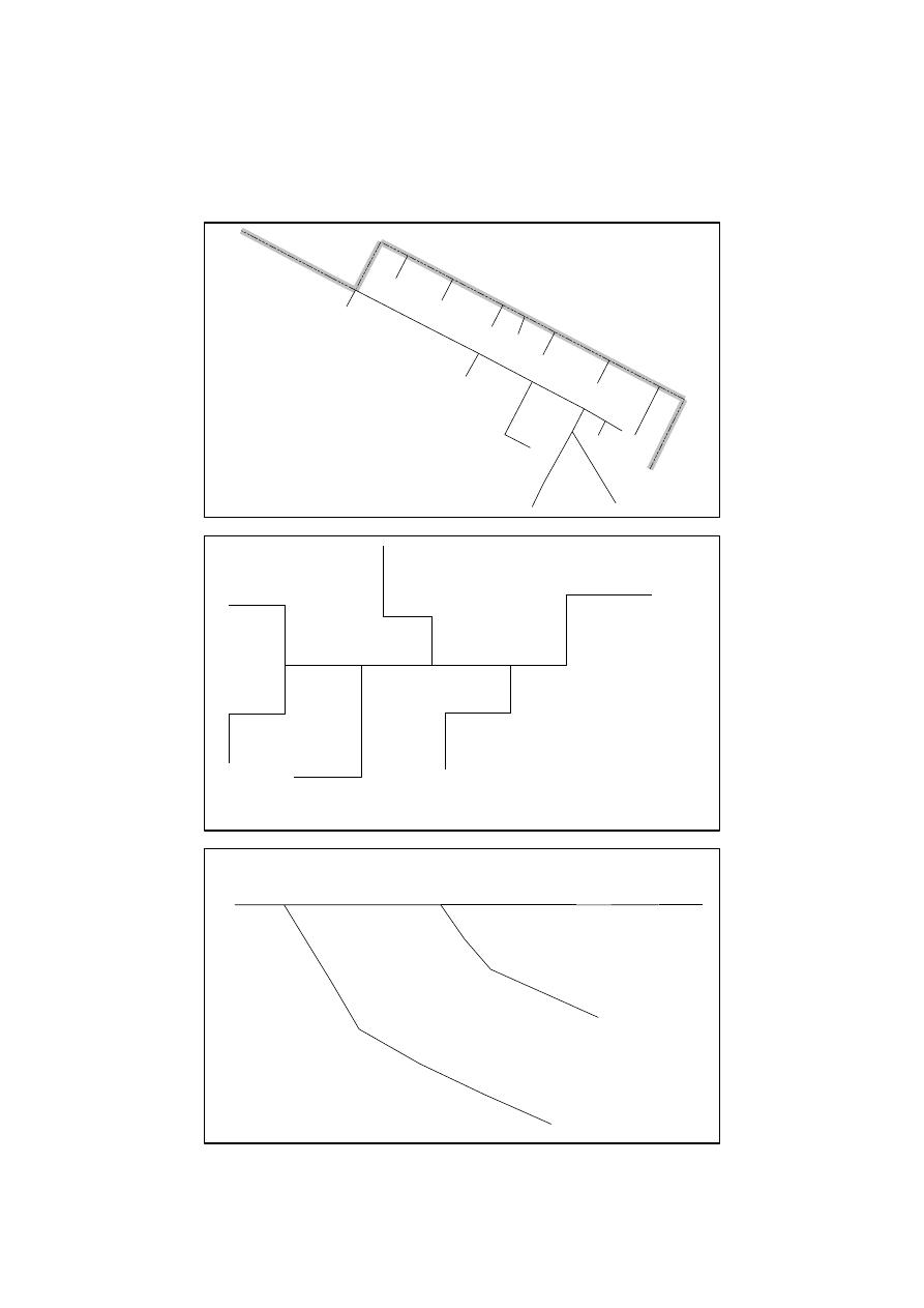
Figure 1. Sewer networks used for the analyses: (A) Mini-Chicó network; (B) Mays and Wenzel [13]
network and (C) Kerman city network.
3.2. Design Constraints
!
!
!
!
!
!
!
!
!
!
!
!
!
!
!
!
!
!
!
!
!
!
!
!
!
!
!
!
!
!
!
!
!
!
!
!
5
4
8
9
13
1
14
19
6
17
25
21
16
11
18
3
2
26
7
10
20
12
34
15
28
27
32
24
23
30
31
22
29
35
33
!
!
!
!
!
!
!
!
!
!
!
!
!
!
!
!
!
!
!
!
!
9
6
4
5
8
2
7
1
3
15
12
19
13
11
18
10
16
14
17
20
!
!
!
!
!
!
!
!
!
!
!
!
!
!
!
!
!
!
!
!
!
3
9
2
8
6
1
5
7
4
15
16
14
17
13
20
12
19
18
11
10
Mini-Chico
No. Nodes: 36
No. Pipes: 35
Ground Elevation [m]: 2551.42 - 2590.20
Pipe Flow [L/s]: 60.00 - 6430.00
Mays and Wenzel (1976)
No. Nodes: 21
No. Pipes: 20
Ground Elevation [m]: 135.60 - 152.40
Pipe Flow [L/s]: 113.20 - 2661.70
Kerman city
No. Nodes: 21
No. Pipes: 20
Ground Elevation [m]: 64.50 - 74.60
Pipe Flow [L/s]: 21.10 - 165.90
A)
B)
C)
Figure 1.
Sewer networks used for the analyses: (A) Mini-Chicó network; (B) Mays and Wenzel [
13
]
network and (C) Kerman city network.
Water 2019, 11, 1148
6 of 12
3.2. Design Constraints
Each network is designed considering the constraints shown in Table
2
and using the optimal
design methodology proposed by Duque et al. [
12
]. As Table
2
shows, the minimum self-cleansing
velocity and minimum shear stress constraints are presented as a range since they depend on the value
(criterion) chosen in Table
1
. Likewise, pipe diameters of 200, 250, 300, 350, 380, 400, 450, 500, 530, 600,
700, 800, 900, 1000, 1050, 1200, 1350, 1400, 1500, 1800, 2200, 2500, 2800, and 3000 mm are assumed
available for those sewer network designs.
The values of all constraint variables are presented in Table
2
. These values are used in the
optimization methodology presented here. As in the case of a cost model, the methodology presented
here is generic in the sense that other constraints used by di
fferent water utilities can be used instead.
A number of self-cleansing criteria are used in three case studies, these are shown as follows (see
Table
1
): (1), (3), (6), (10), and (13). The chosen criteria, cover a range of variation of the minimum velocity
and minimum shear stress criteria applied to stormwater sewer systems, established by water utilities in the
USA, Europe, and Latin America, i.e., minimum velocity
= (0.60–0.90) m/s and shear stress = (2.0–4.0) Pa.
Self-Cleansing Limits
Equations (3) and (4) are used to estimate the impact of several self-cleansing criteria on the
design of sewer networks. A simple general step-by-step procedure to obtain the self-cleansing limits
is considered as follows:
1.
Select a minimum velocity or minimum shear stress from Table
1
;
2.
Select a pipe diameter;
3.
Define the filling ratio
y
D
;
4.
Solve Equation (3), for the minimum velocity, or Equation (4), for shear stress, to estimate the
minimum self-cleansing slope;
5.
Move to the next pipe diameter and repeat step 4;
6.
Move to the next self-cleansing criterion in Table
1
and start the entire procedure over again.
By applying the previous step-by-step procedure, it is possible to obtain several self-cleansing
thresholds for each criterion. These results can be seen in the lines of Figure
2
.
Water 2019, 11, x FOR PEER REVIEW
9 of 14
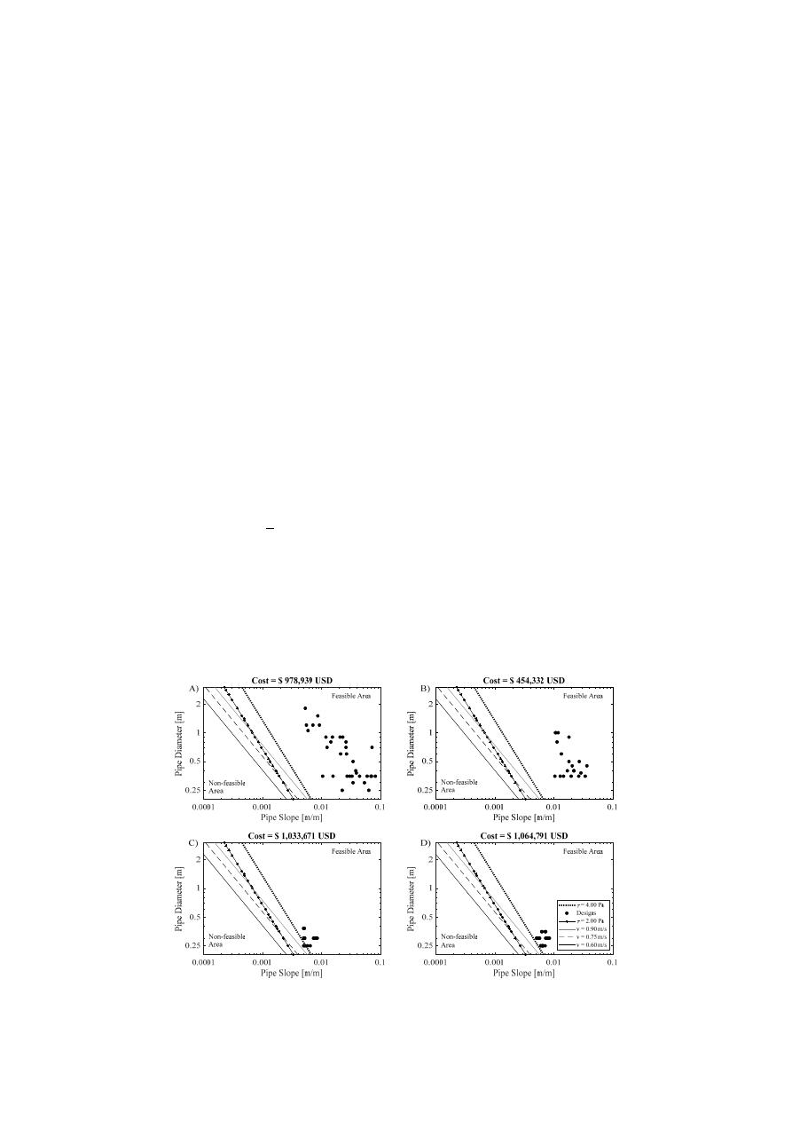
Figure 2. Design results and total costs for the three networks: (A) Mini-Chicó, (B) Mays and Wenzel
[13], (C) Kerman city Design I, and (D) Kerman city Design II.
The results in Figure 2 show a relationship between the design flow of the pipes, the ground
elevation (or terrain slope), and the self-cleansing criteria. In networks with high flow rates and
highly variable ground elevation, such as the Mini-Chicó and Mays and Wenzel [13] stormwater
networks (Figure 2B), pipe designs are always above the self-cleansing restrictions limit, or in the
feasible area, when highly self-cleansing constraining criteria such as 4.0 Pa are used. However,
networks with low flow rates and little topographic difference, such as the wastewater Kerman city
network, are affected by the self-cleansing restriction, and costs will be higher when the criteria are
more restrictive.
The above analysis of the results of the case studies made it necessary to perform a sensitivity
analysis on the design of the network, with the objective to identify limit flow rates and limit terrain
slopes. This sensitivity analysis seeks to evaluate scenarios with low flow rates (wastewater sewer
networks) and low ground elevation differences to determine the relevance of self-cleansing criteria
under these circumstances.
5. Sensitivity Analysis
On the basis of the results of the previous section, a sensitivity analysis is performed considering
only the main path of the Mini-Chicó network, i.e., the highlighted path shown in Figure 1A. The
ground elevation and the inflow rate of each node in this path are modified. It is carried out to find
the limit where self-cleansing criteria, even highly constraining criteria, does not change the final cost
of the optimal sewer network design. This analysis is performed for wastewater sewer system
conditions only, since the purpose is to assess the behavior of low design flow rates under different
topographic conditions.
In the context of this information, five simulations, where different combinations of flow rates
and terrain topography, i.e., ground elevation, are analyzed. For each simulation, a constant inflow
and a variable ground elevation in each node of the main path of the Mini-Chicó network are
assumed. For example, in the first scenario of the first simulation, each node has a constant inflow of
1 L/s, and its ground elevation does not change, compared to the original ground elevation of the
Figure 2.
Design results and total costs for the three networks: (A) Mini-Chicó, (B) Mays and Wenzel [
13
],
(C) Kerman city Design I, and (D) Kerman city Design II.

Water 2019, 11, 1148
7 of 12
3.3. Design Procedure
The procedure for designing sewer networks using Duque et al. [
12
] methodology is as follows:
1.
Create a .txt file that includes the manholes of the main path of the network. Each manhole must
include ground elevation and inflow information;
2.
Define design constraints and list of available commercial diameters;
3.
Create a graph with all the possible arcs (pipes). Each arc has an associated pipe diameter as well
as upstream and downstream elevation to calculate the slope;
4.
Calculate the cost of each pipe using Equation (1);
5.
Calculate the hydraulic of each arc, i.e., determine flow, hydraulic radius, wetted area, and top
width, amongst other hydraulic parameters, using the Manning equation using Equation (3).
If the arc does not fulfill all the design constraints it will not be created;
6.
Use the Bellman–Ford algorithm to estimate the combination of arcs that minimize network cost;
7.
Report the results of the slope and diameter of each pipe in the network.
The previous procedure is applied to each network in Figure
1
. The results of the best combination
of slope versus pipe diameter for each consecutive manhole are presented as dots in Figure
2
.
4. Results and Discussion
The optimal designs for three sewer networks are presented in Figure
2
. These designs compare
and analysis the influence of different self-cleansing criteria on the final cost of the networks. Figure
2
shows the threshold (i.e., the line) for each self-cleansing criterion considered. Each threshold represents
the minimum self-cleansing slope (S
o
in Equations (3) and (4)) for each commercially available diameter.
In addition, Figure
2
shows that the minimum self-cleansing velocity criteria tends to be less restrictive
for large diameters (D
> 1.0 m). As well, the minimum shear stress of 4.0 Pa is clearly more restrictive
than the minimum self-cleansing velocities. In contrast, the minimum shear stress of 2.0 Pa tends to be
less restrictive than the minimum self-cleansing velocities in small sewers (D
< 1.0 m). The threshold
line for a shear stress value of 2.0 Pa intersects the minimum velocities thresholds of 0.9 m
/s and 0.75 m/s
close to diameters of 1.0 m and 0.45 m, respectively. These intersections are produced by the nature of the
equations used to calculate the minimum self-cleansing slope, according to Equations (3) and (4).
As seen in Figure
2
, the results (i.e., each dot in Figure
2
shows the best combination of slope vs
diameter of each pipe in the network, estimated by the methodology used) of the Mini-Chicó and
Mays and Wenzel [
13
] networks (Figure
2
A,B), which are stormwater sewer networks, show that
self-cleansing restrictions are not a critical parameter in the optimal design of these systems, since all
points (i.e., network pipes) are located in the feasible area (i.e., region of graph where all the possible
combinations of diameter and slope of each pipe fulfills the self-cleansing criteria). In this case, the final
cost is the same for all the self-cleansing restrictions.
However, in the case of the Kerman city network designs (Figure
2
C,D), the self-cleansing restrictions
have an impact on the final design of the network. As a result, two different designs are obtained: first,
for the minimum velocities
/shear stresses of 0.6 m/s, 0.75 m/s, 0.9 m/s, and 2.0 Pa (Figure
2
C); and second,
for the minimum shear stress of 4.0 Pa (Figure
2
D). The final cost of the network is calculated using
Equation (1) and increases when a self-cleansing restriction of 4.0 Pa is used. This means that the diameter
or the slope of the pipes increases, as compared with designs obtained with the least restrictive criteria,
to satisfy the hydraulic constraints. On the basis of previously mentioned information, it is possible to
conclude that the final optimal design of a wastewater sewer network, i.e., networks with low inflows per
node, depends on the self-cleansing criterion used in the design.
The results in Figure
2
show a relationship between the design flow of the pipes, the ground
elevation (or terrain slope), and the self-cleansing criteria. In networks with high flow rates and highly
variable ground elevation, such as the Mini-Chicó and Mays and Wenzel [
13
] stormwater networks
(Figure
2
B), pipe designs are always above the self-cleansing restrictions limit, or in the feasible area,

Water 2019, 11, 1148
8 of 12
when highly self-cleansing constraining criteria such as 4.0 Pa are used. However, networks with low
flow rates and little topographic di
fference, such as the wastewater Kerman city network, are affected
by the self-cleansing restriction, and costs will be higher when the criteria are more restrictive.
The above analysis of the results of the case studies made it necessary to perform a sensitivity
analysis on the design of the network, with the objective to identify limit flow rates and limit terrain
slopes. This sensitivity analysis seeks to evaluate scenarios with low flow rates (wastewater sewer
networks) and low ground elevation di
fferences to determine the relevance of self-cleansing criteria
under these circumstances.
5. Sensitivity Analysis
On the basis of the results of the previous section, a sensitivity analysis is performed considering
only the main path of the Mini-Chicó network, i.e., the highlighted path shown in Figure
1
A. The ground
elevation and the inflow rate of each node in this path are modified. It is carried out to find the limit
where self-cleansing criteria, even highly constraining criteria, does not change the final cost of the optimal
sewer network design. This analysis is performed for wastewater sewer system conditions only, since the
purpose is to assess the behavior of low design flow rates under different topographic conditions.
In the context of this information, five simulations, where di
fferent combinations of flow rates and
terrain topography, i.e., ground elevation, are analyzed. For each simulation, a constant inflow and
a variable ground elevation in each node of the main path of the Mini-Chicó network are assumed.
For example, in the first scenario of the first simulation, each node has a constant inflow of 1 L
/s,
and its ground elevation does not change, compared to the original ground elevation of the network.
Accordingly, pipe one of the path will have a design flow rate of 1 L
/s and a ground elevation of
2587.34 m and 2575.50 m at the upstream and downstream nodes, respectively (as shown in Table S4,
in the Supplementary Material). Following this idea, pipe two will have a design flow of 2 L
/s and a
ground elevation of 2575.50 m and 2569.69 m in the upstream and downstream node, respectively,
and this is repeated until the last pipe is reached. Another example is the second scenario of the first
simulation, where the ground elevation is 50% of the original conditions. In this case, the ground
elevation of each node of the path is multiplied by 0.5 and the design flow is the same as compared
to case one of the first scenario, which means the first pipe now has a ground elevation of 1293.67 m
for the upstream node and 1287.75 m for the downstream node. The five proposed simulations are
presented in the Supplementary Material, Tables S4–S8.
The proposed methodology is applied to the defined scenarios. This methodology takes into
account the self-cleansing criteria (3), (4), (6), (9), (11), and (12) shown in Table
1
, which are used for
wastewater sewer systems, and it covers the range of self-cleansing criteria for variations of these
systems. The results of the methodology for each simulation are presented in Figure
3
.
For the wastewater sewer system case, it is found that as slopes decrease, network costs vary
depending on the self-cleansing criteria considered. This suggests that the optimal design is not
independent of self-cleansing criteria. In scenario one of the first simulation, where the terrain
slopes are relatively high, i.e., greater than 1.8%, as shown in Figure
3
A, sewer design costs are
independent of self-cleansing criteria because there is no variation on the cost for the considered criteria.
However, for other scenarios of the same simulation, as slopes decrease, e.g., scenario 3 (terrain slope
of 0.53%) to scenario 5 (terrain slope of 0.09%), the network costs variability becomes larger, depending
on the self-cleansing criteria considered.
On the basis of the results, it is possible to propose a power regression between mean terrain
slope and the inflow per node. The purpose of this regression is to establish the limit conditions on
which costs change as a function of self-cleansing restrictions for sewer system designs. Figure
4
presents the relationship between inflow per node and terrain slope in the main path of the analyzed
network. The horizontal axis represents the mean terrain slope, while the vertical axis represents
the inflow per node in the network. As a result, the dots in Figure
4
indicate the combination of
terrain slope and inflow per node in which self-cleansing criteria do not modify the final cost of
Water 2019, 11, 1148
9 of 12
the network. Consequently, designing with a criterion of 0.6 m
/s for minimum velocity, or 2.0 Pa
for minimum shear stress, is irrelevant. The potential regression curve is generated using the dots
described previously. It is found that the self-cleansing threshold can be estimated with the equation,
inflow per node
=
0.0615 × terrain slope
−0.718
.
Water 2019, 11, x FOR PEER REVIEW
10 of 14
network. Accordingly, pipe one of the path will have a design flow rate of 1 L/s and a ground
elevation of 2587.34 m and 2575.50 m at the upstream and downstream nodes, respectively (as shown
in Table S4, in the Supplementary Material). Following this idea, pipe two will have a design flow of
2 L/s and a ground elevation of 2575.50 m and 2569.69 m in the upstream and downstream node,
respectively, and this is repeated until the last pipe is reached. Another example is the second scenario
of the first simulation, where the ground elevation is 50% of the original conditions. In this case, the
ground elevation of each node of the path is multiplied by 0.5 and the design flow is the same as
compared to case one of the first scenario, which means the first pipe now has a ground elevation of
1293.67 m for the upstream node and 1287.75 m for the downstream node. The five proposed
simulations are presented in the Supplementary Material, Tables S4–S8.
The proposed methodology is applied to the defined scenarios. This methodology takes into
account the self-cleansing criteria (3), (4), (6), (9), (11), and (12) shown in Table 1, which are used for
wastewater sewer systems, and it covers the range of self-cleansing criteria for variations of these
systems. The results of the methodology for each simulation are presented in Figure 3.
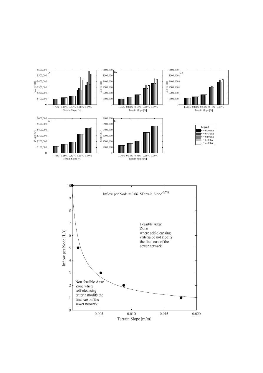
Figure 3. Network costs for the five wastewater proposed simulations: (A) Simulation 1 (Inflow per
node 1 L/s), (B) Simulation 2 (Inflow per node 2 L/s), (C) Simulation 3 (Inflow per node 3 L/s), (D)
Simulation 4 (Inflow per node 5 L/s), and (E) Simulation 5 (Inflow per node 10 L/s). Cost in (USD).
For the wastewater sewer system case, it is found that as slopes decrease, network costs vary
depending on the self-cleansing criteria considered. This suggests that the optimal design is not
independent of self-cleansing criteria. In scenario one of the first simulation, where the terrain slopes
are relatively high, i.e., greater than 1.8%, as shown in Figure 3A, sewer design costs are independent
of self-cleansing criteria because there is no variation on the cost for the considered criteria. However,
for other scenarios of the same simulation, as slopes decrease, e.g., scenario 3 (terrain slope of 0.53%)
to scenario 5 (terrain slope of 0.09%), the network costs variability becomes larger, depending on the
self-cleansing criteria considered.
On the basis of the results, it is possible to propose a power regression between mean terrain
slope and the inflow per node. The purpose of this regression is to establish the limit conditions on
which costs change as a function of self-cleansing restrictions for sewer system designs. Figure 4
presents the relationship between inflow per node and terrain slope in the main path of the analyzed
network. The horizontal axis represents the mean terrain slope, while the vertical axis represents the
inflow per node in the network. As a result, the dots in Figure 4 indicate the combination of terrain
slope and inflow per node in which self-cleansing criteria do not modify the final cost of the network.
Consequently, designing with a criterion of 0.6 m/s for minimum velocity, or 2.0 Pa for minimum
shear stress, is irrelevant. The potential regression curve is generated using the dots described
Figure 3.
Network costs for the five wastewater proposed simulations: (A) Simulation 1 (Inflow
per node 1 L
/s), (B) Simulation 2 (Inflow per node 2 L/s), (C) Simulation 3 (Inflow per node 3 L/s),
(D) Simulation 4 (Inflow per node 5 L
/s), and (E) Simulation 5 (Inflow per node 10 L/s). Cost in (USD).
Water 2019, 11, x FOR PEER REVIEW
11 of 14
previously. It is found that the self-cleansing threshold can be estimated with the equation,
inflow per node = 0.0615 × terrain slope
.
.
Figure 4. Self-cleansing limits in sewer systems.
Figure 4 shows the region where the self-cleansing criteria should be taken into account in the
design for future sewer systems. For example, if the design of a new sewer network has an inflow
rate per node greater than of 3.0 L/s and an average terrain slope of 0.01, the network will always
satisfy all the self-cleansing restrictions, and the final cost will not depend on the criterion used.
However, if the network has the same inflow rate and an average terrain slope of 0.001, the final cost
changes and this change would depend on the self-cleansing restriction used. This figure is useful for
a preliminary evaluation of the impact of self-cleansing criteria on future sewer systems designs. As
shown in Figure 4, pipes located above the dotted line will always have velocities and shear stress
values greater than the minimum required by water utilities to prevent sediment deposition on sewer
pipes, even the most difficult. On the other hand, if the pipes are below the dotted line, the final cost
will be different if a highly restrictive criterion, such as 2.0 Pa or 0.6 m/s, is used.
6. Conclusions
The impact of choosing self-cleansing criteria on the optimal design of sewer networks is
presented in this paper. The impact evaluation of these criteria is carried out using an optimal sewer
network design methodology by Duque et al. [12], subject to a number of design constraints. Three
sewer networks were designed using this methodology taking into consideration several different
self-cleansing criteria based on both minimum flow velocities and shear stresses.
The results obtained demonstrate that the influence of self-cleansing criteria on sewer systems
optimal design depends mainly on the relationship between the land topography and the inflow (i.e.,
design) rate at each node of the network.
Figure 4.
Self-cleansing limits in sewer systems.

Water 2019, 11, 1148
10 of 12
Figure
4
shows the region where the self-cleansing criteria should be taken into account in the
design for future sewer systems. For example, if the design of a new sewer network has an inflow rate
per node greater than of 3.0 L
/s and an average terrain slope of 0.01, the network will always satisfy all
the self-cleansing restrictions, and the final cost will not depend on the criterion used. However, if the
network has the same inflow rate and an average terrain slope of 0.001, the final cost changes and this
change would depend on the self-cleansing restriction used. This figure is useful for a preliminary
evaluation of the impact of self-cleansing criteria on future sewer systems designs. As shown in
Figure
4
, pipes located above the dotted line will always have velocities and shear stress values greater
than the minimum required by water utilities to prevent sediment deposition on sewer pipes, even the
most di
fficult. On the other hand, if the pipes are below the dotted line, the final cost will be different if
a highly restrictive criterion, such as 2.0 Pa or 0.6 m
/s, is used.
6. Conclusions
The impact of choosing self-cleansing criteria on the optimal design of sewer networks is
presented in this paper. The impact evaluation of these criteria is carried out using an optimal
sewer network design methodology by Duque et al. [
12
], subject to a number of design constraints.
Three sewer networks were designed using this methodology taking into consideration several di
fferent
self-cleansing criteria based on both minimum flow velocities and shear stresses.
The results obtained demonstrate that the influence of self-cleansing criteria on sewer systems
optimal design depends mainly on the relationship between the land topography and the inflow (i.e.,
design) rate at each node of the network.
More specifically, the results obtained demonstrate that stormwater sewer system designs (case
studies Mini-Chicó network and Mays and Wenzel [
13
] network) are not a
ffected by the self-cleansing
criteria. The reason for this, is that flow rates in these networks are high during precipitation events,
resulting in velocities and shear stresses above the minimums required, regardless of the self-cleansing
criteria used. In contrast, in wastewater sewer systems where the design flow rates are lower,
self-cleansing criteria becomes relevant for the optimal network design.
Sewer networks with flat topography are also a
ffected by the self-cleansing criteria used for their
design. By applying a highly restrictive self-cleansing criterion, the cost of the network will be higher
compared to a less restrictive criterion. In addition, in sewer pipes with design flow and terrain
slopes greater than 10 L
/s and 0.09%, respectively, the design will remain the same since self-cleansing
restrictions do not a
ffect the final design cost.
A graph depicting self-cleansing limits in sewer systems is presented in the paper (see Figure
4
).
This graph is useful for evaluating new sewer network designs. The designer must include the
information for each pipe in the network (as a point in this graph), to determine if the self-cleansing
restrictions should be considered in the optimal design or not. This is especially important in
low-income areas because by using the graph in Figure
4
it is possible to determine if the construction
of a gravity-based system is viable.
Finally, traditional self-cleansing criteria consider the variability of inflow at each node, i.e., non-steady
flow conditions. Using the design flow rate, the self-cleansing conditions must be satisfied for the
design flow. During lower flow rates, it is possible that particles deposit at the bottom of the pipes,
however, when the design flow is reached all particles deposited are flushed and the pipe is cleaned.
Therefore, the conclusions of this paper will be the same if other design flow rates are considered.
For future work, it is recommended that the proposed methodology be extended to larger sewer
networks and take into account di
fferent cost models. Additionally, this extension should be applied
in the estimation of the layout of the network, i.e., the flow directions and the initial nodes, which have
the most influence on the optimal design of the sewers.

Water 2019, 11, 1148
11 of 12
Supplementary Materials:
The following are available online at
http:
//www.mdpi.com/2073-4441/11/6/1148/s1
,
Table S1: Data for Mini-Chicó sewer network, Table S2. Data for Mays and Wenzel [
13
] network, Table S3. Data for
‘Kerman’ city network. Taken from Afshar et al. [
34
], Table S4. First simulation scenario for the sensitivity analysis,
Table S5. Second simulation scenario for the sensitivity analysis, Table S6. Third simulation scenario for the
sensitivity analysis, Table S7. Fourth simulation scenario for the sensitivity analysis, Table S8. Fifth simulation
scenario for the sensitivity analysis.
Author Contributions:
Conceptualization, C.M., Z.K. and J.S.; Methodology, C.M. and J.S.; Software, C.M.;
Validation, J.S. and Z.K.; Formal Analysis, C.M., Z.K. and J.S.; Investigation, C.M. and J.S.; Resources,
J.S.; Data Curation, C.M.; Writing-Original Draft Preparation, C.M.; Writing-Review & Editing, C.M., Z.K.
and J.S.; Visualization, C.M.; Supervision, Z.K. and J.S.; Project Administration, J.S.; Funding Acquisition,
No Funding Acquisition.
Funding:
This research received no external funding.
Conflicts of Interest:
The authors declare no conflict of interest.
References
1.
Argaman, Y.; Shamir, U.; Spivak, E. Design of Optimal Sewerage Systems. J. Environ. Eng. Div. 1973, 99,
703–716.
2.
Mein, W. Design of Sanitary Sewer Systems by Dynamic Programming. Master’s Thesis, McMaster University,
Hamilton, ON, Canada, 1975.
3.
Li, G.; Matthew, R. New Approach for Optimization of Urban Drainage Systems. J. Environ. Eng. 1990, 116,
927–944. [
CrossRef
]
4.
Holland, M. Computer Models of Wastewater Collection Systems. Master’s Thesis, Harvard University,
Cambridge, MA, USA, 1966.
5.
Elimam, A.A.; Charalambous, C.; Ghobrial, F.H. Optimum Design of Large Sewer Networks. J. Environ. Eng.
1989
, 115, 1171–1190. [
CrossRef
]
6.
Walters, G.; Lohbeck, T. Optimal Layout of Tree Networks Using Genetic Algorithms. Eng. Optim. 1993, 22,
27–48. [
CrossRef
]
7.
Afshar, M. Application of a Genetic Algorithm to Storm Sewer Network Optimization. Sci. Iran. 2006, 13,
234–244.
8.
Cisty, M. Hybrid Genetic Algorithm and Linear Programming Method for Least-Cost Design of Water
Distribution Systems. Water Resour. Manag. 2010, 24, 1–24. [
CrossRef
]
9.
Cozzolino, L.; Cimorelli, L.; Covelli, C.; Mucherino, C.; Pianese, D. An Innovative Approach for Drainage
Network Sizing. Water 2015, 7, 546–567. [
CrossRef
]
10.
Hassan, W.; Jassem, M.; Mohammed, S. A GA-HP Model for the Optimal Design of Sewer Networks.
Water Resour. Manag. 2018, 32, 865–879. [
CrossRef
]
11.
Shao, Z.; Zhang, X.; Li, S.; Deng, S.; Chai, H. A Novel SWMM Based Algorithm Application to Storm Sewer
Network Design. Water 2017, 9, 747. [
CrossRef
]
12.
Duque, N.; Duque, D.; Saldarriaga, J. A New Methodology for the Optimal Design of Series of Pipes in Sewer
Systems. J. Hydroinformatics 2016, 18, 757–772. [
CrossRef
]
13.
Mays, L.W.; Wenzel, H.G. Optimal Design of Multilevel Branching Sewer Systems. Water Resour. Res. 1976,
12, 913–917. [
CrossRef
]
14.
Ebtehaj, I.; Bonakdari, H.; Sharifi, A. Design Criteria for Sediment Transport in Sewers Based on Self-Cleansing
Concept. J. Zhejiang Univ. Sci. A 2014, 15, 914–924. [
CrossRef
]
15.
ATV-DVWK-Regelwerk.
Hydraulische Dimensionierung Und Leistungsnachweis von Abwasserkanalen
Und-Leitungen; AVT-DVWK-A 110; Gesellschaft zur Förderung der Abwassertechnik e.V. (GFA): Hennef,
Germany, 2001.
16.
Vongvisessomjai, N.; Tingsanchali, T.; Babel, M. Non-Deposition Design Criteria for Sewers with Part-Full
Flow. Urban Water J. 2010, 7, 61–77. [
CrossRef
]
17.
Montes, C.; Bohórquez, J.; Borda, S.; Saldarriaga, J. Criteria of Minimum Shear Stress vs. Minimum Velocity
for Self-Cleaning Sewer Pipes Design. Procedia Eng. 2017, 186, 69–75. [
CrossRef
]
18.
Lysne, D. Hydraulic Design of Self-Cleaning Sewage Tunnels. J. Sanit. Eng. Div. Am. Soc. Civ. Eng. 1969, 95,
17–36.
Water 2019, 11, 1148
12 of 12
19.
American Society of Civil Engineers (ASCE). Water pollution control federation. Design and Construction of
Sanitary and Storm Sewers. In American Society of Civil Engineers Manuals and Reports on Engineering Practices;
ASCE: Reston, VA, USA, 1970.
20.
Yao, K. Sewer Line Design Based on Critical Shear Stress. J. Environ. Eng. Div. 1974, 100, 507–520.
21.
Minister of Interior. Instruction Technique Relative Aux Réseaux d’assainissement Des Agglomerations; Circulaire
Interministerielle IT 77284 I; Minister of Interior: Paris, France, 1977.
22.
British Standard Institution. Sewerage-Guide to New Sewerage Construction BS8005 Part 1; British Standard
Institution: London, UK, 1987.
23.
Instituto Ecuatoriano de Normalización. CPE INEN 005-9-1 (1992): Código Ecuatoriano de La Construcción
C.E.C. Normas Para Estudio y Diseño de Sistemas de Agua Potable y Disposición de Aguas Residuales Para Poblaciones
Mayores a 1 000 Habitantes; INEN: Quito, Ecuador, 1992.
24.
European Standard EN 752-4. Drain and Sewer System Outside Building: Part 4. Hydraulic Design and
Environmental Considerations; European Comitte for Standardization (CEN): Brussels, Belgium, 1997.
25.
Great Lakes. Recommended Standars for Wastewater Facilities; Health Education Services Division, Health
Research Inc.: Menands, NY, USA, 2004.
26.
Comisión Nacional del Agua. Manual de Agua Potable, Alcantarillado y Saneamiento; Comisión Nacional del
Agua: Coyoacán, México, 2007.
27.
Instituto Boliviano de Normalización y Calidad. Diseño de Sistemas de Alcantarillado Sanitario y Pluvial (NB
688); Instituto Boliviano de Normalización y Calidad: La Paz, Bolivia, 2007.
28.
Empresas Públicas de Medellín. Guía Para El Diseño Hidráulico de Redes de Alcantarillado; Empresas Públicas
de Medellín: Medellín, Colombia, 2009.
29.
Colombia, Ministerio de Vivienda, Ciudad y Territorio. Reglamento Técnico Del Sector de Agua Potable y
Saneamiento Básico: TÍTULO D. Sistemas de Recolección y Evacuación de Aguas Residuales Domésticas y Aguas
Lluvias; Colombia, Ministerio de Vivienda, Ciudad y Territorio: Bogotá, Colombia, 2012.
30.
Bellman, R. On a Routing Problem. Q. Appl. Math. 1958, 16, 87–90. [
CrossRef
]
31.
Maurer, M.; Scheidegger, A.; Herlyn, A. Quantifying Costs and Lengths of Urban Drainage Systems with a
Simple Static Sewer Infrastructure Model. Urban Water J. 2013, 10, 268–280. [
CrossRef
]
32.
Moeini, R.; Afshar, M. Sewer Network Design Optimization Problem Using Ant Colony Optimization
Algorithm and Tree Growing Algorithm. In Proceedings of the EVOLVE—A Bridge between Probability, Set
Oriented Numerics, and Evolutionary Computation IV, Leiden, The Netherlands, 10–13 July 2013.
33.
Marchionni, V.; Lopes, N.; Mamouros, L.; Covas, D. Modelling Sewer Systems Costs with Multiple Linear
Regression. Water Resour. Manag. 2014, 28, 4415–4431. [
CrossRef
]
34.
Afshar, M.; Shahidi, M.; Rohani, M.; Sargolzaei, M. Application of Cellular Automata to Sewer Network
Optimization Problems. Sci. Iran. 2011, 18, 304–312. [
CrossRef
]
© 2019 by the authors. Licensee MDPI, Basel, Switzerland. This article is an open access
article distributed under the terms and conditions of the Creative Commons Attribution
(CC BY) license (http:
//creativecommons.org/licenses/by/4.0/).
