
water
Article
A Direct Approach for the Near-Optimal Design of
Water Distribution Networks Based on Power Use
Juan Saldarriaga
1,
* , Diego Páez
2
, Camilo Salcedo
1
, Paula Cuero
3
, Laura Lunita López
3
,
Natalia León
3
and David Celeita
3
1
Department of Civil and Environmental Engineering, Universidad de los Andes, Bogotá 111711, Colombia;
ca.salcedo959@uniandes.edu.co
2
Department of Civil Engineering, Queen’s University, Kingston, ON K7L 3N6, Canada;
da.paez270@gmail.com
3
Water Supply and Sewer Systems Research Center (CIACUA), Universidad de los Andes, Bogotá 111711,
Colombia; pa.cuero38@uniandes.edu.co (P.C.); ll.lopez28@uniandes.edu.co (L.L.L.);
n.leon40@uniandes.edu.co (N.L.); da.celeita10@uniandes.edu.co (D.C.)
*
Correspondence: jsaldarr@uniandes.edu.co; Tel.:
+57-1-339-49-49 (ext. 2805)
Received: 7 February 2020; Accepted: 24 March 2020; Published: 6 April 2020
Abstract:
In recent years, iterative computational techniques have been considered as the most
e
ffective methods to tackle the problem of Water Distribution System (WDS) minimum-cost design.
Given their stochastic nature, these approaches involve a large number of hydraulic simulations in
order to obtain suitable results. Herein, a WDS design methodology based entirely on hydraulic
principles is presented. This methodology, named Optimal Power Use Surface (OPUS), focuses on
both reaching low-cost designs and diminishing the number of hydraulic executions (iterations),
by establishing e
fficient ways in which energy is dissipated and flow is distributed throughout the
system. The algorithm was tested in four well known benchmark networks, previously reported
in the literature. OPUS proved that following hydraulic principles is a fair choice to design WDS,
showing plenty of potential in other water distribution mathematical modeling applications and
o
ffering an alternative for the extensive search process undertaken by metaheuristics.
Keywords:
minimum cost design; energy-based methods; optimization; WDS; hydraulic behavior
1. Introduction
The optimal design of Water Distribution Systems (WDS) has been addressed internationally
during the last decades. This is as a result of the need to make an e
fficient distribution of scarce economic
resources without compromising the welfare of society. This problem is substantially magnified in
the context of developing countries because the availability of resources is very limited, and there is
a significant deficiency of WDSs that are capable of supplying water in appropriate conditions. To
overcome these di
fficulties, it is important to use methodologies that are both efficient and effective in
addressing the minimum-cost WDS design problem.
For instance, in developing countries it is common to find some cities that have WDS that cannot
supply water continuously for 24 h a day. Thus, water utilities must find alternative ways to solve the
water availability problem with intermittent water supply, which is not well-solved internationally [
1
].
Another problem found in developing countries is related to aging water networks, but few economic
resources are available to perform proper maintenance and rehabilitation programs. In addition, there
is increasing pressure on water supply because of climate change and population growth [
2
]: cities
are requiring more water, but water is becoming scarcer. Hence, water utilities must find strategies
to solve the problem. For instance, it is well-known that pressure control strategies over all of the
Water 2020, 12, 1037; doi:10.3390
/w12041037
www.mdpi.com
/journal/water

Water 2020, 12, 1037
2 of 26
network allows for reducing energy losses in water networks, as a workaround for making better use
of energy resources. This reduces both energy consumption at pumping stations and water losses in
pipes [
2
], which will allow water utilities to extend the lifespan of aging assets through the reduction
of head-losses. Furthermore, the optimal selection of diameters for the equipment, pipes and pumps in
WDSs have been found to achieve considerable energy reductions [
3
]. This increases the importance of
making good decisions regarding energy losses in the network, as the objective of water distribution is
to deliver water in the quantity required at adequate pressures with the maximum coverage possible
at a
ffordable costs [
3
].
For all these reasons, we find that it is important for water utilities to have several alternatives
for the design of WDSs. As there is very little research on intermittent water supply, there is also a
general lack in design methods that are straightforward and simple enough to be used by water utilities
that lack the interest, the technology or the understanding required to apply state-of-the art design
methods based on evolutionary algorithms. Thus, we propose this methodology as a workaround to
solve design problems using an energy method, which will allow the designer to fully understand
and control what is happening with the energy losses in the network, which we believe may be very
useful to network designers in cities with few computation resources available, or cities where energy
reduction is the main goal.
It has been shown that finding the optimal configuration of diameters is a NP-Hard problem
(non-deterministic polynomial-time) [
4
], even for the simplest of branched networks, it is a highly
constrained nonlinear optimization problem because of the need to satisfy node pressure and pipe
flow restrictions. This means that finding an optimal solution using exhaustive and deterministic
methods is not viable, hence, approximate methods are required to reach near optimal solutions. Most
approximate methodologies are stochastic in nature, and currently most researchers use evolutionary
algorithms. However, those approximate methodologies will try to search the whole solution space to
find optimal and near-optimal solutions, making it necessary to reduce the search space and guide the
heuristic methods to find the solution. For instance, Wu (2005) proposed self-adaptive penalties with
Genetic Algorithms [
5
] and Montalvo (2010) proposed self-adaptive penalties with Particle Swarm
Optimization [
6
].
So far, several authors have proposed approaches to solve the aforementioned problem, which have
led to less expensive designs. In the 1970s and 1980s, engineers used traditional optimization methods
such as enumeration [
7
], linear and nonlinear programming [
8
]. However, in the mid 1990s and
beginnings of the 20th century, these approaches were slowly replaced by metaheuristic algorithms
due to the greater ease of their implementation, more extensive exploration of the solution space,
less dependence on the initial condition of the system, and the ability to integrate the discrete-sized
diameter restrictions. Among the successful attempts in the literature, there are: Di
fferential Evolution
Algorithms [
9
], Genetic Algorithms [
10
], Simulated Annealing ([
11
,
12
]), Harmony Search [
13
], Scatter
Search [
14
], Cross Entropy [
15
], and Particle Swarm [
16
]. Moreover, other authors have proposed
combined approaches such as binary linear programming with di
fferential evolution algorithm [
17
], as
well as proposed approaches to increase the e
fficiency of the algorithm by reducing the search space,
using afterwards a Genetic Algorithm [
18
].
Despite the advantages of these stochastic algorithms, they have an intrinsic limitation that exist
in the requirement of an appropriate determination of several parameters inherent to each algorithm,
which is a time-consuming and laborious task [
19
]. To accomplish this, metaheuristics use a large
number of randomly-generated alternatives and use generic learning functions that progressively
produce better results. However, these algorithms require the assessment of thousands of di
fferent
design alternatives before they converge on a solution. For WDSs, testing each of these alternatives
involves the use of a calculation engine, such as EPANET [
20
]. Thus, the computational e
ffort required
is considerable in most cases. For this reason, the number of iterations executed to obtain the final
design of the WDS may be considered as an indicator of the e
fficiency of the tested methodologies.

Water 2020, 12, 1037
3 of 26
One approach overshadowed by the rapid growth of metaheuristic techniques was based on the
analysis of optimized designs for simple networks, to produce criteria that, combined with hydraulic
principles, could produce optimized results in more complex systems. One of the first examples of this
approach was Wu [
21
], who analyzed the behavior of the cost function in a series of pipes with uniform
demands, establishing a criterion that indicates the target head-loss value for each pipe in the system
to produce a minimum cost design. Featherstone and El-Jumaily [
22
] extended Wu’s criterion by
suggesting its application to looped networks using the Euclidean distance as the main factor to assign
the target Hydraulic Grade Line (HGL) at each node and, therefore, the target head-loss value per pipe.
Based on the contributions of the aforementioned authors, the Optimal Power Use Surface (OPUS)
methodology was first presented by Takahashi et al. [
23
], as a design methodology based on the target
HGL criterion and the use of other hydraulic criteria to extend the concept to looped networks.
This paper describes the OPUS methodology for the optimal design of WDSs and tests its
performance in di
fferent benchmark networks (Hanoi, Balerma, Taichung and Pescara). Several
operational criteria, such as water quality, reliability and environmental impact, can be considered
in an optimization problem related to WDS design and management. However, as a first step in
the development on this alternative type of design method, the objective function considered in this
manuscript is reduced to the construction costs of the system. A comparison against well tested
metaheuristic algorithms shows promising results, both in the performance of the algorithm, as well
as in the understanding of the physical principles of WDS design. The latter makes OPUS a suitable
method for use in decision making at an urban scale, and can be easily understood by engineers.
Finally, based on the obtained results, conclusions and future work guidelines are stated.
OPUS methodology, described in this paper, has become the basis for several applications to
demand-driven models considering di
fferent topologies [
24
], and in pressure-driven models [
25
].
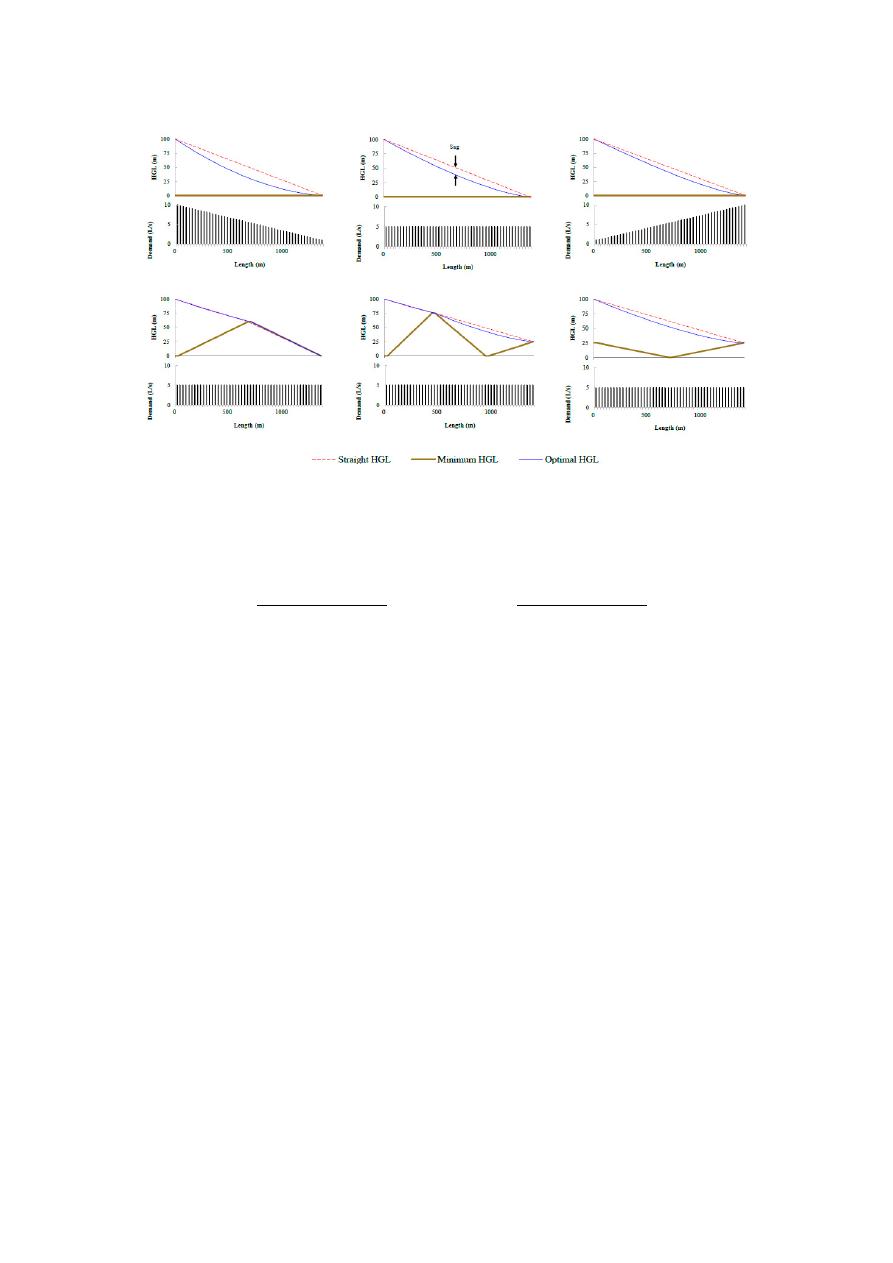
2. Optimal Hydraulic Grade Line (HGL) Criteria
Wu [
21
] analyzed the HGL generated by the global optimum design of pipes in a series system
(drip irrigation main lines). He found that for flat topography, the optimal HGL was always a convex
function. To characterize the function, Wu [
21
] used the straight HGL between the source and the last
demand node, and defined the “sag” as the distance between that straight line and the function at
the middle section. For his case study with uniform demands, the optimal sag was 15% of the total
available head.
Using the linear programming method described by Alperovits and Shamir [
8
], it is possible to
extend Wu’s [
21
] results for di
fferent demand distributions along the series of pipes, as well as different
topography. As can be seen in Figure
1
, the optimal HGL is always a convex function or a combination
of adjacent convex functions with limits at nodes with high elevation (i.e., higher than the straight
HGL). In these figures, the minimum HGL is composed of the elevation along the pipe series and the
minimum pressure allowable. Hence, these figures show di
fferent combinations between topographic
profiles and demand patterns.
Water 2020, 12, 1037
4 of 26
Water 2020, 12, x FOR PEER REVIEW
4 of 26
Figure 1. Comparison of Hydraulic Grade Lines (HGL) resulting from Different Demand
Configurations and Minimum HGL.
A quadratic equation can be adjusted to the convex function found by Wu [21], as shown in
Equation (1):
𝐻𝐺𝐿(𝑥) = 4𝐹 ×
(𝐻𝐺𝐿
− 𝐻𝐺𝐿
)
𝐿
× (𝑥 ) − (1 + 4𝐹) ×
(𝐻𝐺𝐿
− 𝐻𝐺𝐿
)
𝐿
× 𝑥 + 𝐻𝐺𝐿
(1)
where, HGL(x) is the hydraulic grade line at a distance x from the source, HGL
Max
is the hydraulic
grade line at the source, HGL
Min
is the HGL at the final node and represents the minimum value
allowable, F is the predefined sag as a percentage of (HGL
Max
− HGL
Min
), and L is the total length of
the series [26].
Featherstone and El-Jumaily [22] extended the concept of optimal hydraulic grade line to lopped
networks by setting x as the Euclidean distance from each node to the source, and L as the maximum
value of x in the network (i.e., the furthest node). Using the Euclidean distance is a quick approach to
extend Wu’s concept, but clearly the water needs to flow through longer distances according to the
layout of the network. The OPUS methodology introduces a new method to define x and L using the
topological distance in looped networks according to a cost-benefit optimal spanning tree.
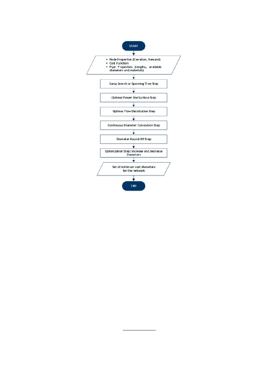
3. Methodology
The Optimal Power Use Surface (OPUS) design methodology is composed of six steps, which
are focused on understanding the flow of energy along the network. These steps are summarized in
the flowchart shown in Figure 2, and described in detail in the subsequent sections.
Figure 1.
Comparison of Hydraulic Grade Lines (HGL) resulting from Di
fferent Demand Configurations
and Minimum HGL.
A quadratic equation can be adjusted to the convex function found by Wu [
21
], as shown in
Equation (1):
HGL
(
x
) =
4F ×
(
HGL
max
− HGL
min
)
L
2
×
x
2
−
(
1
+
4F
)
×
(
HGL
max
− HGL
min
)
L
× x
+
HGL
max
(1)
where, HGL(x) is the hydraulic grade line at a distance x from the source, HGL
Max
is the hydraulic grade
line at the source, HGL
Min
is the HGL at the final node and represents the minimum value allowable, F
is the predefined sag as a percentage of (HGL
Max
− HGL
Min
), and L is the total length of the series [
26
].
Featherstone and El-Jumaily [
22
] extended the concept of optimal hydraulic grade line to lopped
networks by setting x as the Euclidean distance from each node to the source, and L as the maximum
value of x in the network (i.e., the furthest node). Using the Euclidean distance is a quick approach to
extend Wu’s concept, but clearly the water needs to flow through longer distances according to the
layout of the network. The OPUS methodology introduces a new method to define x and L using the
topological distance in looped networks according to a cost-benefit optimal spanning tree.
3. Methodology
The Optimal Power Use Surface (OPUS) design methodology is composed of six steps, which are
focused on understanding the flow of energy along the network. These steps are summarized in the
flowchart shown in Figure
2
, and described in detail in the subsequent sections.
Water 2020, 12, 1037
5 of 26
Water 2020, 12, x FOR PEER REVIEW
5 of 26
Figure 2. Optimal Power Use Surface (OPUS) methodology flow chart.
3.1. Sump Search or Spannin Tree Structure
The sump search, or the identification of the Spanning Tree structure, is based on two hydraulic
principles: (1) In a least-cost WDS, the demand at the nodes should be supplied by transporting the
water from the sources using a single route, and (2) As the pipes flow rates for design purposes
increase, the marginal costs diminish.
For the first principle, it can be stated that redundancy is hydraulically inefficient, despite its
benefits in terms of reliability. As a result, branched WDSs can manage to be less expensive compared
to looped networks; thus, this step aims to decompose the looped system into an open tree-like
structure. This leads to the identification of nodes in the original network that can be considered as
sumps of a fictional branched network, meaning the nodes with the lowest hydraulic head among all
its neighbors.
The second principle is based in the analysis of the relationship between the pipe diameter and
its cost per length unit. A typical equation to represent the constructive cost of a pipe is given by
Equation (2)
:
𝐶𝑜𝑠𝑡 = 𝐾 × 𝐿 × 𝑑
(2)
where, 𝐶𝑜𝑠𝑡 is the cost of pipe 𝑖; 𝐾 is the coefficient of the cost function; 𝐿 is the length of pipe 𝑖; 𝑑
is the diameter assigned to pipe 𝑖; and 𝑥 is the exponent of the cost function [21]. On the other hand,
Hazen-Williams friction head losses equation relates to pipe diameters, friction head losses and
flowrates as shown in Equation (3):
ℎ =
10.67 × 𝐿 × 𝑄
.
𝐶
.
× 𝑑
.
(3)
Figure 2.
Optimal Power Use Surface (OPUS) methodology flow chart.
3.1. Sump Search or Spannin Tree Structure
The sump search, or the identification of the Spanning Tree structure, is based on two hydraulic
principles: (1) In a least-cost WDS, the demand at the nodes should be supplied by transporting the
water from the sources using a single route, and (2) As the pipes flow rates for design purposes increase,
the marginal costs diminish.
For the first principle, it can be stated that redundancy is hydraulically ine
fficient, despite its
benefits in terms of reliability. As a result, branched WDSs can manage to be less expensive compared to
looped networks; thus, this step aims to decompose the looped system into an open tree-like structure.
This leads to the identification of nodes in the original network that can be considered as sumps of a
fictional branched network, meaning the nodes with the lowest hydraulic head among all its neighbors.
The second principle is based in the analysis of the relationship between the pipe diameter and
its cost per length unit. A typical equation to represent the constructive cost of a pipe is given by
Equation (2):
Cost
i
=
K × L
i
× d
x
i
(2)
where, Cost
i
is the cost of pipe i; K is the coe
fficient of the cost function; L
i
is the length of pipe i;
d
i
is the diameter assigned to pipe i; and x is the exponent of the cost function [
21
]. On the other
hand, Hazen-Williams friction head losses equation relates to pipe diameters, friction head losses and
flowrates as shown in Equation (3):
h
f i
=
10.67 × L
i
× Q
1.85
i
C
1.85
× d
4.87
i
(3)
Water 2020, 12, 1037
6 of 26
where, h
f i
is the head-loss along pipe i (m), Q
i
represents the volumetric flowrate on pipe i (m
3
/s
)
and
C is the pipe roughness coe
fficient (dimensionless). Therefore, by solving Equation (3) for d
i
and then
replacing it in Equation (2), an expression for the cost of the pipe as a function of Q
i
is obtained, as
shown in Equation (4):
CostQ
(
Q
i
) =
Cost
i
=
K
0
× L
i
×
Q
i
S
0.54
f i
x/2.63
(4)
where, K
0
=
K ×
10.67
C
1.85
x/4.87
; and S
f i
is the friction slope for pipe i defined by h
f i
/L
i
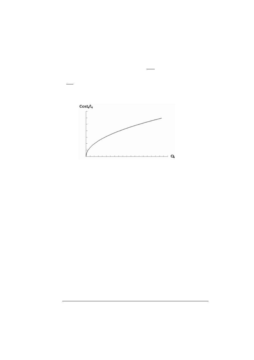
. Figure
3
shows
the trend of this new expression, where it is shown that for typical values of x (lower than 2.63),
the marginal cost decreases as the design flowrate of a pipe increases.
Water 2020, 12, x FOR PEER REVIEW
6 of 26
where, ℎ is the head-loss along pipe 𝑖 (m), 𝑄 represents the volumetric flowrate on pipe 𝑖 (𝑚 /𝑠)
and 𝐶 is the pipe roughness coefficient (dimensionless). Therefore, by solving Equation (3) for 𝑑 and
then replacing it in Equation (2), an expression for the cost of the pipe as a function of 𝑄 is obtained,
as shown in Equation (4):
𝐶𝑜𝑠𝑡𝑄(𝑄 ) = 𝐶𝑜𝑠𝑡 = 𝐾
×
𝐿
×
𝑄
𝑆
.
/ .
(4)
where, 𝐾 = 𝐾 ×
.
.
/ .
; and 𝑆 is the friction slope for pipe 𝑖 defined by ℎ /𝐿 . Figure 3 shows
the trend of this new expression, where it is shown that for typical values of 𝑥 (lower than 2.63), the
marginal cost decreases as the design flowrate of a pipe increases.
Figure 3. Schematic relation between pipe cost and flow.
Considering that WDS are represented as a set of junctions and links, the problem of obtaining
a tree-like structure for the WDS is similar to the problem of finding a Minimum Spanning Tree (MST)
for a weighted undirected graph. In this problem, the vertices of the graph are the nodes of the WDS,
while the edges of the graph are the pipes (links) in the WDS. Prim [27] proposed an algorithm to
find the MST that minimizes the sum of link lengths. For the OPUS methodology, Prim’s Algorithm
can be modified to maximize a recursively updated Benefit-Cost (𝐵/𝐶) value for every link in the
minimum spanning tree. This is equivalent to finding the MST for a graph weighted with the 𝐵/𝐶
values, but with the 𝐵/𝐶 values updated at each iteration of Prim’s Algorithm.
The spanning tree is initialized at the water source and grows by incorporating nodes from the
selection front (set of adjacent nodes that are not yet connected to the spanning tree), ensuring the
connection performed reaches the highest 𝐵/𝐶 value possible among its set. This procedure is
repeated until every node (demand and not demand nodes) in the network is connected to the tree.
If there is more than one water source in the network, there will be the same number of trees as
sources in the system, since there should exist only one route to supply each node in the spanning
tree structure. In that case, a tree will be initialized per water source, and the selection front will
include any node not yet connected to a tree but adjacent to one.
The 𝐵/𝐶 function of adding a pipe-node pair 𝑖 in the selection front, is calculated as the ratio
between the demand of the node added to the tree and the marginal cost associated with its
connection to the source [26], as shown in Equation (5). This marginal cost is computed as the sum of
the total cost of the pipe 𝑖 and the cost difference related to the transportation of the additional flow
through all of the upstream pipes [28].
(𝐵/𝐶) =
𝑂𝑢𝑡𝑓𝑙𝑜𝑤
𝐶𝑜𝑠𝑡𝑄(𝑂𝑢𝑡𝑓𝑙𝑜𝑤 ) + ∑
𝐶𝑜𝑠𝑡𝑄 𝐹𝑙𝑜𝑤𝑅𝑎𝑡𝑒 + 𝑂𝑢𝑡𝑓𝑙𝑜𝑤 − 𝐶𝑜𝑠𝑡𝑄(𝐹𝑙𝑜𝑤𝑅𝑎𝑡𝑒 )
∈
(5)
where, (𝐵/𝐶) is the Benefit–Cost value of adding the attached pipe-node pair 𝑖. 𝑂𝑢𝑡𝑓𝑙𝑜𝑤 is the flow
demand of node 𝑖, which is the additional flow conveyed through the network, if pair 𝑖 was added
Figure 3.
Schematic relation between pipe cost and flow.
Considering that WDS are represented as a set of junctions and links, the problem of obtaining a
tree-like structure for the WDS is similar to the problem of finding a Minimum Spanning Tree (MST)
for a weighted undirected graph. In this problem, the vertices of the graph are the nodes of the WDS,
while the edges of the graph are the pipes (links) in the WDS. Prim [
27
] proposed an algorithm to
find the MST that minimizes the sum of link lengths. For the OPUS methodology, Prim’s Algorithm
can be modified to maximize a recursively updated Benefit-Cost (B/C) value for every link in the
minimum spanning tree. This is equivalent to finding the MST for a graph weighted with the B/C
values, but with the B/C values updated at each iteration of Prim’s Algorithm.
The spanning tree is initialized at the water source and grows by incorporating nodes from the
selection front (set of adjacent nodes that are not yet connected to the spanning tree), ensuring the
connection performed reaches the highest B/C value possible among its set. This procedure is repeated
until every node (demand and not demand nodes) in the network is connected to the tree.
If there is more than one water source in the network, there will be the same number of trees as
sources in the system, since there should exist only one route to supply each node in the spanning tree
structure. In that case, a tree will be initialized per water source, and the selection front will include
any node not yet connected to a tree but adjacent to one.
The B/C function of adding a pipe-node pair i in the selection front, is calculated as the ratio
between the demand of the node added to the tree and the marginal cost associated with its connection
to the source [
26
], as shown in Equation (5). This marginal cost is computed as the sum of the total cost
of the pipe i and the cost di
fference related to the transportation of the additional flow through all of
the upstream pipes [
28
].
(
B/C
)
i
=
Out f low
i
CostQ
(
Out f low
i
) +
P
j ∈ Upstream
pipes
h
CostQ
FlowRate
j
+
Out f low
i
− CostQ
FlowRate
j
i
(5)
where,
(
B/C
)
i
is the Benefit–Cost value of adding the attached pipe-node pair i. Out f low
i
is the flow
demand of node i, which is the additional flow conveyed through the network, if pair i was added
Water 2020, 12, 1037
7 of 26
to the tree. FlowRate
j
is the flow that goes through pipe j of the tree before inserting any adjacent
pipe-node pairs. The first term in the denominator of Equation (5) stands for the cost of the new
included pipe, while the sum corresponds to the marginal cost upstream [
26
]. This expression is
computed using Equation (4) as the function CostQ.
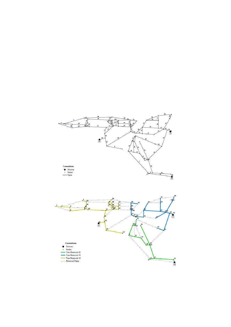
Given Pescara [
29
], the Italian WDS benchmark shown in Figure
4
a, the sump search procedure
will be developed as follows: Starting from the three sources (identified as 15, 43 and 65), each selection
front is analyzed. In other words, the possible link-node pairs that can be added to Reservoir 65
are
<90,76> (i.e., junction 90 and link 76) and <6,89>. Respectively, the link-node pairs <42,54> and
<14,11> could be added to sources 43 and 15. To decide which source will be the root of the first tree,
and consequently, which link–node pair will be added initially to the tree, the B/C value is computed
for each link–node pair, selecting the one that maximizes this criterion. This procedure is repeated
until every node is connected to a tree. In Figure
4
b, the minimum cost-spanning tree is shown for
Pescara WDS, where each link maximized the B/C value at each selection front. Dashed links are those
who were not included in the spanning tree, but are present in the original WDS.
Water 2020, 12, x FOR PEER REVIEW
7 of 26
to the tree. 𝐹𝑙𝑜𝑤𝑅𝑎𝑡𝑒 is the flow that goes through pipe 𝑗 of the tree before inserting any adjacent
pipe-node pairs. The first term in the denominator of Equation (5) stands for the cost of the new
included pipe, while the sum corresponds to the marginal cost upstream [26]. This expression is
computed using Equation (4) as the function 𝐶𝑜𝑠𝑡𝑄.
Given Pescara [29], the Italian WDS benchmark shown in Figure 4a, the sump search procedure
will be developed as follows: Starting from the three sources (identified as 15, 43 and 65), each
selection front is analyzed. In other words, the possible link-node pairs that can be added to Reservoir
65 are <90,76> (i.e., junction 90 and link 76) and <6,89>. Respectively, the link-node pairs <42,54> and
<14,11> could be added to sources 43 and 15. To decide which source will be the root of the first tree,
and consequently, which link–node pair will be added initially to the tree, the 𝐵/𝐶 value is computed
for each link–node pair, selecting the one that maximizes this criterion. This procedure is repeated
until every node is connected to a tree. In Figure 4b, the minimum cost-spanning tree is shown for
Pescara WDS, where each link maximized the 𝐵/𝐶 value at each selection front. Dashed links are
those who were not included in the spanning tree, but are present in the original WDS.
(a)
(b)
Figure 4. (a) Layout of Pescara Water Distribution System (WDS). Pipe ID shown in the labels above
the pipes (b) Minimum-Cost Spanning Tree. Node ID shown in the labels. Dashed links correspond
to the pipes that do not form part of the spanning tree.
Figure 4.
(a) Layout of Pescara Water Distribution System (WDS). Pipe ID shown in the labels above
the pipes (b) Minimum-Cost Spanning Tree. Node ID shown in the labels. Dashed links correspond to
the pipes that do not form part of the spanning tree.

Water 2020, 12, 1037
8 of 26
In particular, it must be noted that as the Pescara network is supplied by three di
fferent sources, it
is expected that this tree-structure identification step will reach three di
fferent branched sub-systems,
each one fed by a unique source. In general terms, for systems with n sources, the nodes in the original
network will be grouped into a maximum number of n di
fferent tree structures. This is accomplished
by seeking to maximize the B/C relationship and ensuring that every node in the original network is
assigned to a tree, except for the reservoirs that can be isolated given their B/C relationship. Hence,
for further steps in this methodology, the obtained trees are considered simultaneously.
Moreover, the values involved in this step are not actual costs, but values obtained proportionally
from the relation presented in Figure
3
. Configuring the tree using this cost-benefit function has an
O(NN
2
) time complexity, where NN is the number of nodes. At the end, the status of the last nodes in
each branch is set to ‘sumps’, which will be useful for the rest of the methodology [
28
].
3.2. Optimal Power Use Surface (OPUS)
The entire methodology is named after this specific step due to the close relation with the work
developed by Wu [
21
]. This step consists of assigning a target HGL to each node in the network,
which determines the head-losses for each pipe in advance [
26
].
In the proposed algorithm, the OPUS is computed using the tree structure, described in the
previous section. Here, the Wu [
21
] concept of target HGL is used by setting the pressure of all of
the sump nodes to the minimum admissible value [
26
], and calculating the intermediate nodes’ head
for each path knowing the head in each reservoir. For this purpose, each node’s topological distance,
measured along the path of pipes that connect the node with the source, must be computed previously.
Then Equation (1) is used to compute the target HGL at every node.
Since Equation (1) depends on the parameter F (sag), a sensitivity analysis to evaluate its e
ffect in
the final design cost was performed. The evaluated range was F ∈
[
0, 0.25
]
. In order to represent a
straight HGL, the minimum value was set to 0, since a negative sag results in a concave down parabolic
HGL, opposite to Wu’s criterion [
26
]. The maximum value of the sag was obtained by finding the
maximum F in Equation (1) that produces a monotonically decreasing HGL for x ∈
[
0, L
]
. It can be
shown that a value of 0.25 is the maximum sag under this consideration (no increasing HGL).
The results of the sensitivity analysis showed that a second-order polynomial could be adjusted to
the cost vs. F relationship. Therefore, the design must be done three times with continuous diameters
and the costs must be calculated to find the optimal target sag of a network. The criteria considered for
the three designs are identical, apart from the general sag used. Subsequently, taking into account that
cost vs. sag is a parabola, the optimal sag is determined by finding the minimum cost of a second-order
polynomial regression obtained by the three cost vs. sag points previously calculated [
26
].
If the three designs are made using F
=
{0, 0.1, 0.25} then the optimal target sag can be computed
using Equation (6):
Optimal sag
=
21C
0
− 25C
0.1
+
4C
0.25
40
(
3C
0
− 5C
0.1
+
2C
0.25
)
(6)
where, C
x
is the cost of the architecture obtained using a sag F
=
x [
26
]. The procedure corresponding
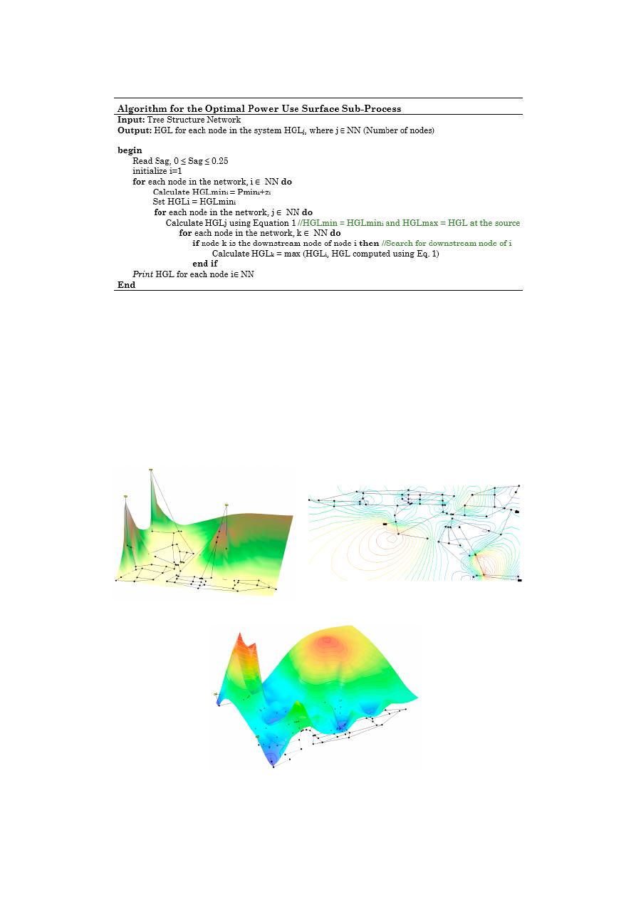
to this step is described in the pseudo-code shown in Figure
5
.
Water 2020, 12, 1037
9 of 26
Water 2020, 12, x FOR PEER REVIEW
9 of 26
Figure 5. Algorithm for OPUS subprocess.
The target sag (𝐹) must be recalculated at each intersection in an upstream analysis through the
network, where the branches converge. In order to do so, the flow is weighted on each downstream
course. It is essential to analyze the nodes with a high elevation, in order to avoid the assignment of
a head value that does not fulfill the pressure demand [26].
The optimal power use surface for the Pescara network is shown in Figure 6 as an example. The
terrain of the network is shown in Figure 6a, while subsequent figures show the level curves for the
HGL (Figure 6b), and its corresponding surface (Figure 6c). Note that, as mentioned before, for the
water source, the HGL corresponds to the total head available in the reservoir, while in the sump
nodes its value was assigned equal to the minimum pressure.
(a) (b)
(c)
Figure 6. (a) Topographic profile for Pescara. (b) Level curve for the HGL. (c) Assigned surface for the
Pescara network.
Figure 5.
Algorithm for OPUS subprocess.
The target sag
(
F
)
must be recalculated at each intersection in an upstream analysis through the
network, where the branches converge. In order to do so, the flow is weighted on each downstream
course. It is essential to analyze the nodes with a high elevation, in order to avoid the assignment of a
head value that does not fulfill the pressure demand [
26
].
The optimal power use surface for the Pescara network is shown in Figure
6
as an example. The
terrain of the network is shown in Figure
6
a, while subsequent figures show the level curves for the
HGL (Figure
6
b), and its corresponding surface (Figure
6
c). Note that, as mentioned before, for the
water source, the HGL corresponds to the total head available in the reservoir, while in the sump nodes
its value was assigned equal to the minimum pressure.
Water 2020, 12, x FOR PEER REVIEW
9 of 26
Figure 5. Algorithm for OPUS subprocess.
The target sag (𝐹) must be recalculated at each intersection in an upstream analysis through the
network, where the branches converge. In order to do so, the flow is weighted on each downstream
course. It is essential to analyze the nodes with a high elevation, in order to avoid the assignment of
a head value that does not fulfill the pressure demand [26].
The optimal power use surface for the Pescara network is shown in Figure 6 as an example. The
terrain of the network is shown in Figure 6a, while subsequent figures show the level curves for the
HGL (Figure 6b), and its corresponding surface (Figure 6c). Note that, as mentioned before, for the
water source, the HGL corresponds to the total head available in the reservoir, while in the sump
nodes its value was assigned equal to the minimum pressure.
(a) (b)
(c)
Figure 6. (a) Topographic profile for Pescara. (b) Level curve for the HGL. (c) Assigned surface for the
Pescara network.
Figure 6.
(a) Topographic profile for Pescara. (b) Level curve for the HGL. (c) Assigned surface for the
Pescara network.

Water 2020, 12, 1037
10 of 26
Once this step is concluded, all nodes must have an objective head value assigned. Thus, a flow
value is required in order to calculate the diameter of each pipe in the network, using the process
explained in the next section.
3.3. Optimal Flow Distribution
In a looped network, the same hydraulic gradient surface can be obtained by combining di
fferent
configurations of diameters when the set of allowable pipe sizes is R
+
(positive real numbers) [
24
].
Thus, this step is intended to find a unique flow distribution in the network that fits to the Optimal
Power Use Surface (OPUS) previously defined, ensuring it satisfies the mass conservation at each node.
Since at this point the objective HGL has been assigned using Wu’s [
16
] criteria with the topological
distance, the spanning tree structure is no longer required. Therefore, for further steps, the described
procedures are done using the original graph (network).
The determination of the optimal flow distribution consists of the division of the flow demand into
the upstream pipes, starting from the sumps. Three di
fferent criteria were explored for this procedure
by Saldarriaga et al. [
19
]:
(1)
Uniform distribution: It assumes that all pipes have the same flow, which is calculated by
dividing the total flow demand of each node into the number of upstream pipes connected to
it [
26
].
(2)
Proportional distribution: For each pipe, the flow distributes proportionally to H
/L
2
, where H
stands for the head losses in the pipe and L for its length.
(3)
All-in-one distribution: The conveyance capacity for all the pipes upstream of the analyzed node
is computed assuming they have the minimum diameter available (d
min
), and they are assigned
as the design flows. If this is insu
fficient to transport the total flow demand, the residual flow is
assigned to the one pipe with highest hydraulic favorability.
Depending on the used criterion, the reliability of the network varies. In this context, the reliability
can be defined as the ability of the system to handle failures, and it can be measured through several
approaches such as the Network Resilience Index (NRI), proposed by Prasad and Park [
30
]. Saldarriaga
et al. [
24
] proved that the reliability of the network is magnified when the uniform distribution is used,
contrasted to the other two criteria. However, in this paper only the All-in-one distribution is considered
as it was found to be the one that produced least-cost networks [
21
].
There are multiple criteria to analyze the appropriateness of di
fferent pipes in order to define the
main pipe, which is the one that transports the largest portion of the total flow demanded. Similar to
the tree structure step, the pipe with the highest flow is determined through a function. This expression
is Equation (7), which refers to the Hydraulic Favorability, where the pipe with the maximum value of
this parameter is chosen. For nonsump nodes, the total demand is computed by adding its flow to the
one required downstream. An Iterative-Recursive Algorithm (IRA) can be applied to perform all of the
calculations with an O(NN) time complexity [
26
].
Hydraulic Favorability
i
=
HGL
up
− HGL
down
L
2
(7)
where, HGL
up
is the hydraulic grade line of the upstream node of pipe i, HGL
down
is the HGL of the
downstream node of pipe i, and L is the length of pipe i [
26
]. At the end of the process, all of the pipes
in the system must have been assigned an objective flow value. The subprocess is explained in detail
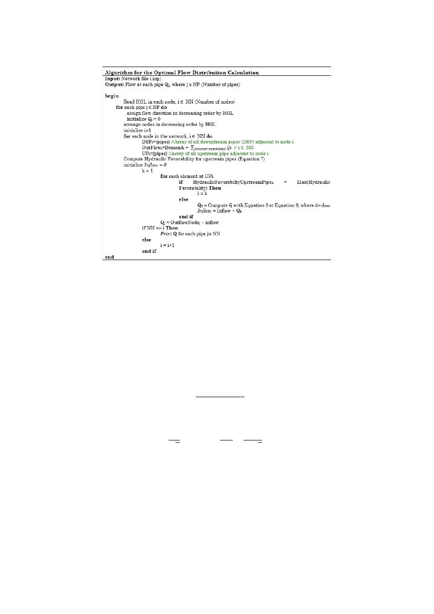
in Figure
7
.
Water 2020, 12, 1037
11 of 26
Water 2020, 12, x FOR PEER REVIEW
11 of 26
Figure 7. Algorithm for the Optimal Flow Distribution.
3.4. Continuous Diameter Calculation
Once the assigned head-losses and the objective flow rate for each pipe are defined, the diameter
required in a continuous range as the hydraulic design can be easily calculated in an explicit manner
using the Hazen-Williams equation (solving for 𝑄 on Equation (3)) and iteratively with the Darcy-
Weisbach and Colebrook-White equations (Equations (8) and (9), respectively) [26]. Then, the
obtained continuous diameter must be rounded to an available size to satisfy the constraints of the
problem and turn an ideal optimal design into a low-cost feasible one.
In this equation, 𝑄 represents the volumetric flowrate (m /s), ℎ is the head loss over the length
of pipe (m), 𝐶 is the pipe roughness coefficient (dimensionless), 𝑑 is the diameter of the pipe (m), and
𝐿 is the length of the pipe (m):
𝑄 =
ℎ × 𝑔 × 𝜋 × 𝑑
8𝑓 × 𝐿
/
(8)
where 𝑔 is the acceleration due to gravity (m/s ), and 𝑓 is the Darcy friction factor (dimensionless).
1
𝑓
= −2 log
𝑘
3.7𝑑
+
2.51
𝑅𝑒 𝑓
(9)
where, 𝑘 is the roughness height of the pipe (m), and 𝑅𝑒 is the Reynolds Number (dimensionless).
3.5. Diameter Round-off
As described before, the continuous diameters obtained in the previous step must be rounded
to satisfy the commercial constraints of the problem. Therefore, in this step the continuous diameter
of each pipe is rounded to a discrete value from the list of commercially available diameter sizes,
which is represented by the set
𝑫
=
{
𝐷
1
, … , 𝐷
𝑁𝐷
}
[26].
During this research, it has been found that using approaches for approximating the diameter
based in either the nearest equivalent flow, as well as the nearest equivalent head-loss led to
promising results. The latter is accomplished by raising the continuous diameter values to a power
Figure 7.
Algorithm for the Optimal Flow Distribution.
3.4. Continuous Diameter Calculation
Once the assigned head-losses and the objective flow rate for each pipe are defined, the diameter
required in a continuous range as the hydraulic design can be easily calculated in an explicit
manner using the Hazen-Williams equation (solving for Q on Equation (3)) and iteratively with the
Darcy-Weisbach and Colebrook-White equations (Equations (8) and (9), respectively) [
26
]. Then,
the obtained continuous diameter must be rounded to an available size to satisfy the constraints of the
problem and turn an ideal optimal design into a low-cost feasible one.
In this equation, Q represents the volumetric flowrate (m
3
/s
)
, h
f
is the head loss over the length
of pipe (m), C is the pipe roughness coe
fficient (dimensionless), d is the diameter of the pipe (m), and L
is the length of the pipe (m):
Q
=
h
f
× g ×
π
2
× d
5
8 f × L
1/2
(8)
where g is the acceleration due to gravity (m/s
2
)
, and f is the Darcy friction factor (dimensionless).
1
p f
=
−2 log
10
k
s
3.7d
+
2.51
Re
p f
(9)
where, k
s
is the roughness height of the pipe (m), and Re is the Reynolds Number (dimensionless).
3.5. Diameter Round-o
ff
As described before, the continuous diameters obtained in the previous step must be rounded to
satisfy the commercial constraints of the problem. Therefore, in this step the continuous diameter of
each pipe is rounded to a discrete value from the list of commercially available diameter sizes, which is
represented by the set D
=
{
D
1
,
. . . , D
ND
} [
26
].
During this research, it has been found that using approaches for approximating the diameter
based in either the nearest equivalent flow, as well as the nearest equivalent head-loss led to promising
results. The latter is accomplished by raising the continuous diameter values to a power of 2.6 for

Water 2020, 12, 1037
12 of 26
the equivalent flow criterion (as explained in the Tree Structure step), or using a power of −4.87 in
the case of the equivalent head-loss criterion. The aforementioned powers describe the relationship
between the head-loss and the diameter, according to the Hazen-Williams equation calculated using the
International System of Units. However, this action has a negative e
ffect on the hydraulic performance
of the network, requiring an additional step to post-optimize the current network.
3.6. Optimization
Finally, the optimization step has two central purposes: (1) To guarantee that all nodes have a
pressure above the minimum required value; and (2) To find possible reductions in the capital cost of
the network. The first objective is achieved by increasing diameters (if needed), setting as a starting
point the ones with larger unit head-loss di
fferences between real and target values [
26
]. The process is
repeated until all the nodes in the system meet the minimum pressure requirement.
The second goal is reached with a double review over the pipes, decreasing the diameters if no
constraint is violated. This two-way review starts at the reservoirs, heading towards the sumps in the
direction of the flow, and then backwards. This means that the need of reducing the pipe’s diameter
is verified twice. If any variation caused a pressure deficit in the system, it is reversed immediately,
otherwise it remains [
28
].
Given that the diameter of one pipe is increased iteratively while some nodes are below the
pressure demand, this step requires the highest percentage of iterations of the whole method because a
hydraulic simulation must be run per pipe for each diameter variation. This single heuristic can be
used alone to accomplish feasible designs, even though, it is strongly dependent on the initial pipe
configuration [
28
].
4. Results and Discussion
The OPUS methodology was tested and validated using four well-known benchmark networks:
Hanoi [
31
], Balerma [
32
], Taichung [
33
] and Pescara [
29
]. Di
fferent configurations of the parameters
defined on each step of the methodology were tested, looking for optimal designs with discrete
diameters (assigning only diameters commercially available). In some cases, there were assigned
continuous values (D
=
R
+
), where D is the diameter of each pipe, to be considered as a theoretical
solution giving the best costs that may be found with the methodology without the restriction of
continuous diameter values. The input files corresponding to the optimal designs reported below are
available in the supplementary files of this research.
4.1. Hanoi
The Hanoi network was first introduced by Fujiwara and Khang [
31
], and it has become a
well-known benchmark WDS for the comparison of design methodologies since its appearance. For
this network the Hazen-Williams equation is used to calculate the friction losses; a Hazen-Williams
coe
fficient of C
=
130 is the value for this benchmark network. For the design process a 30 m minimum
pressure was established and in order to calculate the network total cost, it is necessary to add the costs
of all pipes using a potential function of each diameter. That function has a unit coe
fficient of $1.1/m
and 1.5 as the exponent. The set of available design diameters are 12, 16, 20, 24, 30 and 40 inches [
26
],
and their corresponding unit costs are shown in Table
1
. The network is composed of 34 pipes and
31 nodes configured in 3 loops. The whole system is supplied by 1 reservoir with a constant head of
100 m. A sag value of 0.25 was used in OPUS methodology, while both the layout of the network and
the obtained spanning tree are shown in Figure
8
a.
Table 1.
Unit Costs of Hanoi Network.
Diameter (in.)
12.0
16.0
20.0
24.0
30.0
40.0
Unit Cost ($
/m)
45.73
70.40
98.39
129.33
180.75
278.28
Water 2020, 12, 1037
13 of 26
Water 2020, 12, x FOR PEER REVIEW
13 of 26
(a)
(b)
Figure 8. Cont.
Water 2020, 12, 1037
14 of 26
Water 2020, 12, x FOR PEER REVIEW
14 of 26
(c)
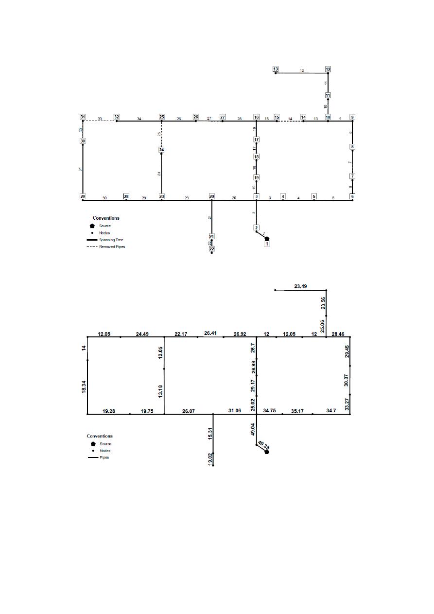
Figure 8. (a) General layout and Spanning Tree for Hanoi Network. Dashed lines are pipes from the
original networks that are not included in the Spanning Tree (b) OPUS design considering continuous
diameters (in inches) (c) OPUS design considering discrete diameters (in inches).
In OPUS, the Hanoi network was tested using continuous diameters, reaching a total cost of
$5,535,888 and the pipe configuration shown in Figure 8b. As can be seen in the mentioned figure,
higher values than the maximum allowable diameter (40 inches according to Fujiwara and Khang
(1990)), are assigned to some pipes of the network. In order to consider the influence of the diameter
restrictions on the final cost of the network, two different discrete designs were performed: the first
one based on the original diameter list, and the second one considering the availability of a 50 inches
diameter.
In the first scenario considering the original diameter list, the OPUS algorithm generated a total
cost of $6,374,525 after 106 iterations, with the resulting pipe diameters (in inches) shown in Figure
8c. These iterations correspond to the total number of hydraulic simulations executed by the
algorithm.
Although this is not the least cost reported, the number of hydraulic simulations needed to reach
this result is three orders of magnitude smaller than that of other approaches, as is shown in Table 2.
In regards to Hanoi, the least cost design used as benchmark was $6.081 million, given that lower
cost results do not satisfy pressure constraints in EPANET2 as shown by [34]. To this end, OPUS
reached a solution that has a difference of 4.81% with respect to the lowest value reported in a very
low number of iterations.
Table 2. Reported costs and number of iterations for the Hanoi WDS.
Algorithm
Cost (millions)
Number of Iterations
Genetic Algorithm [10]
$6.073
1,000,000
Simulated annealing [11]
$6.056
53,000
Harmony search [35]
$6.056
200,000
Shuffled frog leaping [36]
$6.073
26,987
Shuffled complex evolution [37]
$6.220
25,402
Genetic Algorithm [38]
$6.056
18,300
Figure 8.
(a) General layout and Spanning Tree for Hanoi Network. Dashed lines are pipes from the
original networks that are not included in the Spanning Tree (b) OPUS design considering continuous
diameters (in inches) (c) OPUS design considering discrete diameters (in inches).
In OPUS, the Hanoi network was tested using continuous diameters, reaching a total cost of
$5,535,888 and the pipe configuration shown in Figure
8
b. As can be seen in the mentioned figure,
higher values than the maximum allowable diameter (40 inches according to Fujiwara and Khang
(1990)), are assigned to some pipes of the network. In order to consider the influence of the diameter
restrictions on the final cost of the network, two di
fferent discrete designs were performed: the
first one based on the original diameter list, and the second one considering the availability of a 50
inches diameter.
In the first scenario considering the original diameter list, the OPUS algorithm generated a total
cost of $6,374,525 after 106 iterations, with the resulting pipe diameters (in inches) shown in Figure
8
c.
These iterations correspond to the total number of hydraulic simulations executed by the algorithm.
Although this is not the least cost reported, the number of hydraulic simulations needed to reach
this result is three orders of magnitude smaller than that of other approaches, as is shown in Table
2
.
In regards to Hanoi, the least cost design used as benchmark was $6.081 million, given that lower cost
results do not satisfy pressure constraints in EPANET2 as shown by [
34
]. To this end, OPUS reached a
solution that has a di
fference of 4.81% with respect to the lowest value reported in a very low number
of iterations.
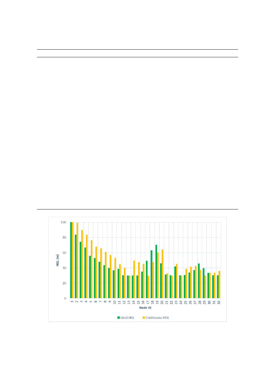
In the second scenario considering the 50” diameter, the total cost of the design obtained following
the OPUS algorithm was of only $5,533,393, due to the closer resemblance between the final hydraulic
gradient surface and the target one, as shown in Figure
9
. In this approach, the unit cost of the 50” pipe
was extrapolated, resulting in a value of $388.91
/m. Finally, the resulting diameters listed by their ID
shown in Figure
8
a are 50, 50, 40, 40, 40, 40, 40, 24, 24, 40, 20, 20, 12, 12, 12, 16, 20, 20, 20, 40, 16, 12, 40,
30, 24, 20, 12, 12, 12, 12, 12, 12, 12 and 20. These diameters are measured in inches.
Water 2020, 12, 1037
15 of 26
Table 2.
Reported costs and number of iterations for the Hanoi WDS.
Algorithm
Cost (millions)
Number of Iterations
Genetic Algorithm [
10
]
$6.073
1,000,000
Simulated annealing [
11
]
$6.056
53,000
Harmony search [
35
]
$6.056
200,000
Shu
ffled frog leaping [
36
]
$6.073
26,987
Shu
ffled complex evolution [
37
]
$6.220
25,402
Genetic Algorithm [
38
]
$6.056
18,300
Ant colony optimization [
39
]
$6.134
35,433
Genetic Algorithms [
32
]
$6.081
50,000
Particle Swarm Optimization [
40
]
$6.093
6600
Genetic Algorithms [
12
]
$6.173
26,457
Simulated annealing [
12
]
$6.333
26,457
Simulated annealing with tabu search [
12
]
$6.353
26,457
Local search with simulated annealing [
12
]
$6.308
26,457
Harmony search [
13
]
$6.081
27,721
Cross entropy [
15
]
$6.081
97,000
Scatter search [
33
]
$6.081
43,149
Modified GA 1 [
41
]
$6.056
18,000
Modified GA 2 [
41
]
$6.190
18,000
Particle swarm harmony search [
16
]
$6.081
17,980
Heuristic based approach [
42
]
$6.701
70
Di
fferential evolution [
43
]
$6.081
48,724
Honey-bee mating optimization [
44
]
$6.117
15,955
Heuristic based approach [
45
]
$6.232
259
Self-adaptive di
fferential evolution [
46
]
$6.081
60,582
Pseudo-Genetic Algorithm [
34
]
$6.081
25,000
Linear Programming – Di
fferential Evolution [
17
]
$6.081
33,148
B-GENOME (B-GA) [
18
]
$6.182
26,000
SOGH [
47
]
$6.337
94
OPUS (This research)
$6.374
106
Water 2020, 12, x FOR PEER REVIEW
15 of 26
Ant colony optimization [39]
$6.134
35,433
Genetic Algorithms [32]
$6.081
50,000
Particle Swarm Optimization [40]
$6.093
6600
Genetic Algorithms [12]
$6.173
26,457
Simulated annealing [12]
$6.333
26,457
Simulated annealing with tabu search [12]
$6.353
26,457
Local search with simulated annealing [12]
$6.308
26,457
Harmony search [13]
$6.081
27,721
Cross entropy [15]
$6.081
97,000
Scatter search [33]
$6.081
43,149
Modified GA 1 [41]
$6.056
18,000
Modified GA 2 [41]
$6.190
18,000
Particle swarm harmony search [16]
$6.081
17,980
Heuristic based approach [42]
$6.701
70
Differential evolution [43]
$6.081
48,724
Honey-bee mating optimization [44]
$6.117
15,955
Heuristic based approach [45]
$6.232
259
Self-adaptive differential evolution [46]
$6.081
60,582
Pseudo-Genetic Algorithm [34]
$6.081
25,000
Linear Programming – Differential Evolution [17]
$6.081
33,148
B-GENOME (B-GA) [18]
$6.182
26,000
SOGH [47]
$6.337
94
OPUS (This research)
$6.374
106
In the second scenario considering the 50” diameter, the total cost of the design obtained
following the OPUS algorithm was of only $5,533,393, due to the closer resemblance between the final
hydraulic gradient surface and the target one, as shown in Figure 9. In this approach, the unit cost of
the 50” pipe was extrapolated, resulting in a value of $388.91/m. Finally, the resulting diameters listed
by their ID shown in Figure 8a are 50, 50, 40, 40, 40, 40, 40, 24, 24, 40, 20, 20, 12, 12, 12, 16, 20, 20, 20,
40, 16, 12, 40, 30, 24, 20, 12, 12, 12, 12, 12, 12, 12 and 20. These diameters are measured in inches.
Figure 9. Comparison between the ideal HGL and that obtained by OPUS considering the additional
50 in. diameter.
Figure 9.
Comparison between the ideal HGL and that obtained by OPUS considering the additional
50 in. diameter.
Water 2020, 12, 1037
16 of 26
4.2. Balerma
The Balerma network corresponds to an irrigation district in Almería, Spain [
32
], and is composed
of a total of 454 pipes and 443 demand nodes which are supplied by 4 reservoirs. The topology of the
network is presented in Figure
10
.
Water 2020, 12, x FOR PEER REVIEW
16 of 26
4.2. Balerma
The Balerma network corresponds to an irrigation district in Almería, Spain [32], and is
composed of a total of 454 pipes and 443 demand nodes which are supplied by 4 reservoirs. The
topology of the network is presented in Figure 10.
(a)
(b)
Figure 10. (a) General layout for Balerma network and the spanning tree obtained for each reservoir,
including the removed pipes. Dashed lines are pipes from the original networks that are not included
in the Spanning Tree (b) OPUS design for Balerma Network. The diameters are shown in millimeters.
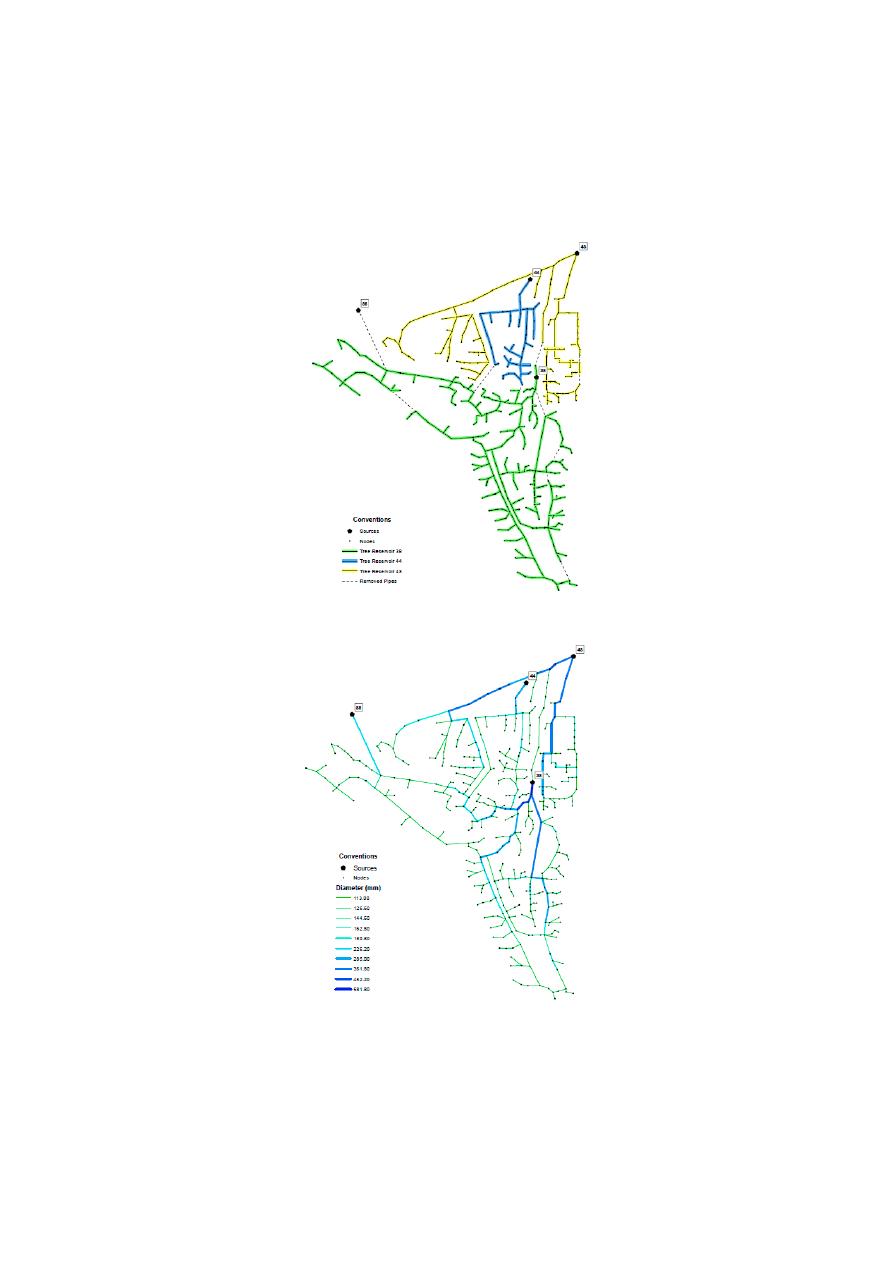
Figure 10.
(a) General layout for Balerma network and the spanning tree obtained for each reservoir,
including the removed pipes. Dashed lines are pipes from the original networks that are not included
in the Spanning Tree (b) OPUS design for Balerma Network. The diameters are shown in millimeters.
The head-loss expression commonly used is the Darcy-Weisbach equation. The pipe diameters
commercially available for its design are manufactured exclusively in PVC, with an absolute roughness

Water 2020, 12, 1037
17 of 26
coe
fficient of 0.0025 mm. The minimum pressure allowable is of 20 m, and it has 10 commercially
available pipes, the costs of which are presented in Table
3
. A sag value of 0.25 was used in the OPUS
methodology, while both the general layout and the obtained spanning tree are shown in Figure
10
a.
In this figure, it is shown that if the network is fed by multiple sources, it will have a maximum of one
spanning tree per reservoir. In this step, all nodes must be assigned to a spanning tree. However, a
reservoir can be isolated given that it is not e
fficient in terms of B/C to feed a part of the network.
Table 3.
Unit costs of Balerma network.
Diameter (mm)
113
126.6
144.6
162.8
180.8
226.2
285
361.8
452.2
581.8
Unit Cost (
€/m)
7.22
9.10
11.92
14.84
18.38
28.60
45.39
76.32
124.64 215.85
Considering continuous diameters for this network, OPUS algorithm generated a design with a
total cost of
€1.755 million. After executing the Round-off and Optimization processes, the optimal
discrete design reached a total cost of
€2.015 million, requiring 1165 hydraulic simulations. The
configuration of diameters in the OPUS design is shown in Figure
10
b. Table
4
shows reported costs
and number of iterations reached by several authors.
Table 4.
Reported costs and number of iterations for the Balerma WDS.
Algorithm
Cost (
€ millions)
Number of Iterations
Genetic algorithm [
32
]
2.302
10,000,000
Harmony search [
13
]
2.601
45,400
Harmony search [
13
]
2.018
10,000,000
Genetic algorithm [
12
]
3.738
45,400
Simulated annealing [
12
]
3.476
45,400
Simulated annealing with tabu search [
12
]
3.298
45,400
Local search with simulated annealing [
12
]
4.310
45,400
Hybrid discrete dynamically dimensioned search [
48
]
1.940
30,000,000
Harmony search with particle swarm [
16
]
2.633
45,400
SOGH [
47
]
2.100
1779
Memetic algorithm [
49
]
3.120
45,400
Genetic heritage evolution by stochastic transmission [
50
]
2.002
250,000
Di
fferential evolution [
46
]
1.998
2,400,000
Self-adaptive di
fferential evolution [
46
]
1.983
1,300,000
OPUS (this study)
2.015
1165
4.3. Taichung
Sung et al. [
28
] introduced the Taichung network, which is a WDS located in a city in Taiwan,
Taichung. This WDS has 31 pipes and 20 nodes, included in 12 di
fferent loops. Water is supplied by
one reservoir with 113.98 m as initial head. Table
5
presents the 13 commercial diameters and their
costs [
26
]. For the design process a minimum head of 15 m was imposed and the friction loss equation
is Hazen-Williams with 100 as the C coe
fficient [
28
]. The network’s topology is shown in Figure
11
a.
The OPUS methodology reached a cost of $8,914,400 after 47 iterations, considering discrete
diameters as shown in Figure
11
b. Reported costs in literature, and its corresponding number of
iterations for Taichung network are shown in Table
6
.
Water 2020, 12, 1037
18 of 26
Table 5.
Unit costs of Taichung network.
Diameter (mm)
Unit Cost (NT Dollar
/m)
100
860
150
1160
200
1470
250
1700
300
2080
350
2640
400
3240
450
3810
500
4400
600
5580
700
8360
800
10,400
900
12,800
Water 2020, 12, x FOR PEER REVIEW
18 of 26
Table 5. Unit costs of Taichung network.
Diameter (mm)
Unit Cost (NT Dollar/m)
100 860
150 1160
200 1470
250 1700
300 2080
350 2640
400 3240
450 3810
500 4400
600 5580
700 8360
800 10,400
900 12,800
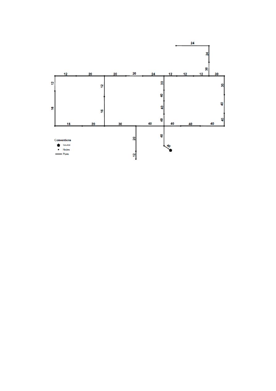
(a) (b)
Figure 11. (a) Spanning Tree for Taichung Network. Dashed lines are pipes from the original networks
that are not included in the Spanning Tree. (b) OPUS design for Taichung Network. The diameters
are shown in millimeters.
The OPUS methodology reached a cost of $8,914,400 after 47 iterations, considering discrete
diameters as shown in Figure 11b. Reported costs in literature, and its corresponding number of
iterations for Taichung network are shown in Table 6.
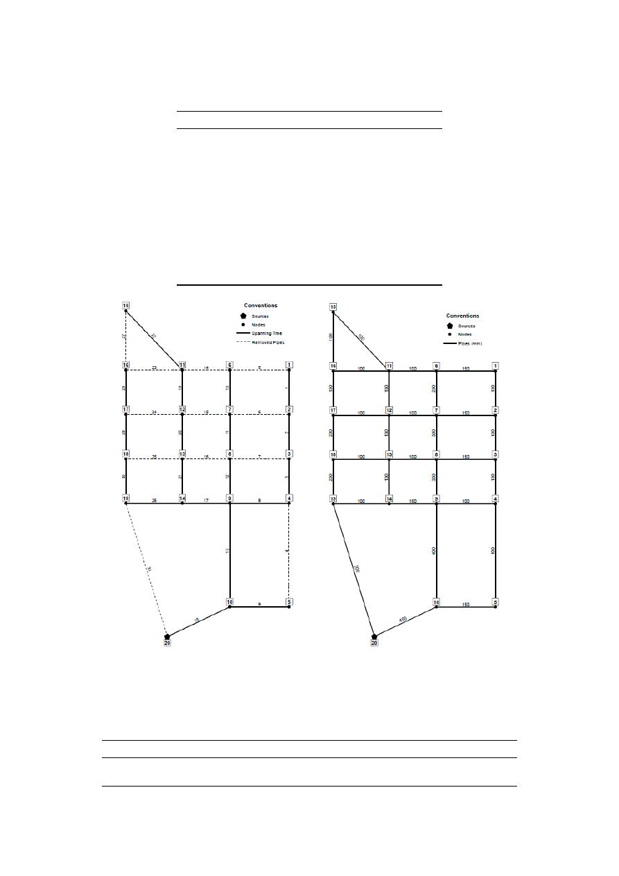
Figure 11.
(a) Spanning Tree for Taichung Network. Dashed lines are pipes from the original networks
that are not included in the Spanning Tree. (b) OPUS design for Taichung Network. The diameters are
shown in millimeters.
Table 6.
Reported costs and number of iterations for the Taichung WDS.
Algorithm
Cost (NT Dollar)
Number of iterations
Tabu search [
33
]
8,774,900
Not Available
OPUS (this study)
8,914,400
47

Water 2020, 12, 1037
19 of 26
4.4. Pescara Network
The Pescara network corresponds to the reduced version of the water distribution system of a
medium-size city at Italy [
29
]. This WDS is composed of three reservoirs with a fixed head ranging
between 53.08 m to 57.00 m, 99 pipes and 68 demand nodes.
The available pipes are made of cast iron represented by a uniform Hazen-Williams roughness
coe
fficient of 130. The unitary costs of the available pipes are shown in Table
7
. A sag value of 0.10
was used in the OPUS methodology. However, for this network the general layout and the obtained
spanning tree for each reservoir are shown in Figure
4
a.
Table 7.
Unit costs of Pescara network.
Diameter (mm)
Unit Cost (
€/m)
100
27.7
125
38
150
40.5
200
55.4
250
75
300
92.4
350
123.1
400
141.9
450
169.3
500
191.5
600
246
700
319.6
800
391.1
The minimum pressure head of all demand nodes must be maintained at 20 m. However, this
system has two additional constraints in its design: A set of maximum pressures at each demand node
ranging between 28.5 m and 55.9 m, and a maximum velocity at each pipe of 2 m
/s.
The OPUS methodology reached an optimal discrete design with a total cost of
€2.161 million,
requiring 206 hydraulic simulations. The configuration of the diameters obtained by OPUS methodology
are shown in Figure
12
a. Table
8
presents minimum costs and the number of iterations reached by
several authors for Pescara Network.
Table 8.
Reported costs and number of iterations for the Pescara WDS.
Algorithm
Cost (
€ millions)
Number of Iterations
Mixed Integer Linear Programming—MILP [
29
]
1.820
Not available—Time limit: 7200 s
OPUS (This research)
2.161
206
The cost obtained using OPUS design is 18.7% higher than the reported by Bragalli et al. [
29
];
however, according to the authors, this result was the best solution they could reach within a time
limit of 7200 s. In terms of computational e
fficiency, OPUS methodology requires 210 iterations,
which represents less than one second in time, using an average desktop computer (we used a
fourth-generation Intel Core i7 processor with 16 GB of RAM, however design software requirements
are lower).
Water 2020, 12, 1037
20 of 26
Water 2020, 12, x FOR PEER REVIEW
20 of 26
(a)
(b) (c)
Figure 12. (a) OPUS design for Pescara Network. The diameters are shown in millimeters. The
resulting spanning tree is shown in Figure 4b. (b) Zoom in to the location of Pipe 84. (c) Zoom in to
the location of Pipe 103.
The cost obtained using OPUS design is 18.7% higher than the reported by Bragalli et al. [29];
however, according to the authors, this result was the best solution they could reach within a time
limit of 7200 seconds. In terms of computational efficiency, OPUS methodology requires 210
iterations, which represents less than one second in time, using an average desktop computer (we
used a fourth-generation Intel Core i7 processor with 16 GB of RAM, however design software
requirements are lower).
Finally, OPUS design fulfilled pressure constraints of the network, considering both the
minimum pressure service as well as the maximum pressures allowable at each node. However, these
results showed that 2 pipes (ID 84 and ID 103, the latter located downstream the reservoir 43 as shown
in Figure 12b,c correspondingly) in the system did not meet the maximum velocity constraint.
Table 8. Reported costs and number of iterations for the Pescara WDS.
Algorithm
Cost (€
millions)
Number of Iterations
Mixed Integer Linear Programming—MILP
[29]
1.820
Not available—Time limit: 7200
seconds
OPUS (This research)
2.161
206
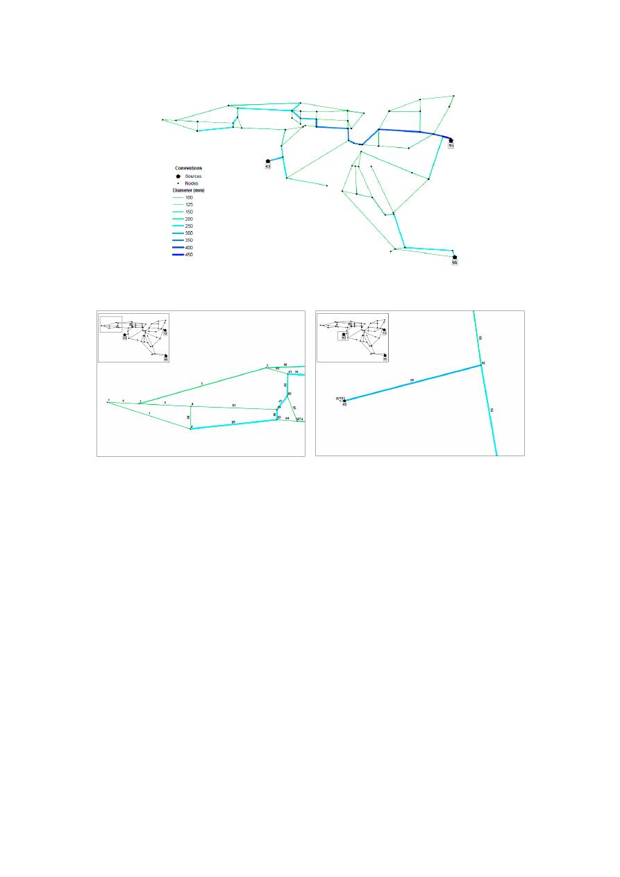
Figure 12.
(a) OPUS design for Pescara Network. The diameters are shown in millimeters. The
resulting spanning tree is shown in Figure
4
b. (b) Zoom in to the location of Pipe 84. (c) Zoom in to the
location of Pipe 103.
Finally, OPUS design fulfilled pressure constraints of the network, considering both the minimum
pressure service as well as the maximum pressures allowable at each node. However, these results
showed that 2 pipes (ID 84 and ID 103, the latter located downstream the reservoir 43 as shown in
Figure
12
b,c correspondingly) in the system did not meet the maximum velocity constraint.
4.5. Sensitivity Analysis OPUS Methodology—Sag
As described in the Optimal Power Use Surface (OPUS) step (Section
3.2
) of this methodology,
the optimal HGL is predefined using the sag, extending Wu (1975) criterion. In this context, the sag is a
positive value between 0.0 and 0.50 that represents the di
fference, in percentage, between a straight
HGL and the parabolic HGL that represents the minimum cost design.
To analyze the sensitivity of the resulting OPUS designs regarding the selected sag, several tests
were developed considering values between 0.0 and 0.5, with increments of 0.05. In order to assess the
performance of the methodology, two indexes were considered in addition to the cost (in millions) of
the resulting designs for measuring the reliability of the system: the Resilience Index (RI) proposed
by Todini [
51
], and the Network Resilience Index (NRI) proposed by Prasad and Park [
30
]. In first
place, the RI measures the capacity to be prepared against the occurrence of sudden failures in the
supply system based on the surplus of energy available at each junction; this is after demands and
pressures have been satisfied. Second, the NRI considers the combined e
ffect of both surplus power
Water 2020, 12, 1037
21 of 26
and reliable loops in the network as a measurement of resilience. NRI addressed the reliable loops as a
consequence of having uniform diameters connected to a node.
In this analysis, Hanoi, Balerma, Taichung and Pescara networks were considered, leading to the
results shown in Figure
13
. As can be seen, in the case of Hanoi and Balerma, the least-cost design is
obtained by using a sag of 0.25. In Taichung, the least-cost design is reached by using a sag value of 0.1
to 0.2, having an increase in the cost of the network of 0.88% when the sag value is 0.15. In Pescara,
the near-optimal design is reached by using a sag value between 0.1 and 0.25. However, when a
sag of 0.20 is used, an increase of 2.05% to the cost is obtained. Hence, it can be concluded that the
least-cost designs are obtained when between 0.10 and 0.25 are used. Accordingly, the behavior shown
by Pescara and Taichung may be a result of the rounding process, where small changes in the optimal
power surface lead to some increase in pipe diameters.
Water 2020, 12, x FOR PEER REVIEW
21 of 26
4.5. Sensitivity Analysis OPUS Methodology
—
Sag
As described in the Optimal Power Use Surface (OPUS) step (Section 3.2) of this methodology,
the optimal HGL is predefined using the sag, extending Wu (1975) criterion. In this context, the sag
is a positive value between 0.0 and 0.50 that represents the difference, in percentage, between a
straight HGL and the parabolic HGL that represents the minimum cost design.
To analyze the sensitivity of the resulting OPUS designs regarding the selected sag, several tests
were developed considering values between 0.0 and 0.5, with increments of 0.05. In order to assess
the performance of the methodology, two indexes were considered in addition to the cost (in millions)
of the resulting designs for measuring the reliability of the system: the Resilience Index (RI) proposed
by Todini [51], and the Network Resilience Index (NRI) proposed by Prasad and Park [30]. In first
place, the RI measures the capacity to be prepared against the occurrence of sudden failures in the
supply system based on the surplus of energy available at each junction; this is after demands and
pressures have been satisfied. Second, the NRI considers the combined effect of both surplus power
and reliable loops in the network as a measurement of resilience. NRI addressed the reliable loops as
a consequence of having uniform diameters connected to a node.
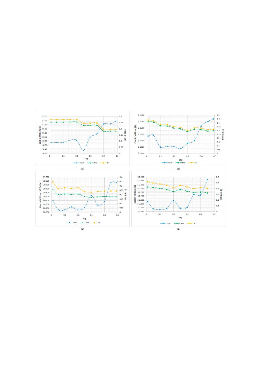
In this analysis, Hanoi, Balerma, Taichung and Pescara networks were considered, leading to
the results shown in Figure 13. As can be seen, in the case of Hanoi and Balerma, the least-cost design
is obtained by using a sag of 0.25. In Taichung, the least-cost design is reached by using a sag value
of 0.1 to 0.2, having an increase in the cost of the network of 0.88% when the sag value is 0.15. In
Pescara, the near-optimal design is reached by using a sag value between 0.1 and 0.25. However,
when a sag of 0.20 is used, an increase of 2.05% to the cost is obtained. Hence, it can be concluded
that the least-cost designs are obtained when between 0.10 and 0.25 are used. Accordingly, the
behavior shown by Pescara and Taichung may be a result of the rounding process, where small
changes in the optimal power surface lead to some increase in pipe diameters.
Figure 13. Sensitivity Results for Cost and Network Resilience Index (NRI) for Different Values of Sag
(a) Hanoi Network. (b) Balerma Network. (c) Taichung Network (d) Pescara Network.
In addition, for sag values higher than 0.25, the total costs of the network will be greater. The
reason for this was first presented by Wu (1975), as for bigger sag values there will be a lower energy
slope upstream (negative sag) or downstream (positive sag). Thus, cost will increase because of the
Figure 13.
Sensitivity Results for Cost and Network Resilience Index (NRI) for Di
fferent Values of Sag
(a) Hanoi Network. (b) Balerma Network. (c) Taichung Network (d) Pescara Network.
In addition, for sag values higher than 0.25, the total costs of the network will be greater. The
reason for this was first presented by Wu (1975), as for bigger sag values there will be a lower energy
slope upstream (negative sag) or downstream (positive sag). Thus, cost will increase because of the
need for use of larger sizes of pipe in those sections. Therefore, the costs curve will be convex, with the
lower values being between the aforementioned range for sag values (0.10 and 0.25 depending on the
network), and increasing above this threshold.
Regarding the comparison between the Resilience Index and the Network Resilience Index, it can
be seen that they both decrease as the sag values increase. Given this, it can be inferred that for sag
values above 0.25, the obtained results will be more expensive and less resilient. In addition, based on
the topology of the networks, it can be seen that if the system tends to be more branched, the NRI
will approach the RI. On the other hand, if the network tends to be more looped, the NRI will di
ffer
considerably from the RI.
The results presented for the Hanoi, Balerma and Pescara networks will be compared with
some results available in literature to validate the performance of OPUS methodology in terms of the
resilience of the network. As is presented in Figure
13
, the Hanoi network has values ranging from 0.19

Water 2020, 12, 1037
22 of 26
to 0.27 for the RI and 0.18–0.26 for the NRI. Similarly, the Balerma network has a RI between 0.30–0.44,
and an NRI between 0.28 and 0.42. Finally, Pescara network has a RI ranging between 0.39 to 0.52,
and an NRI between 0.32–0.43.
Several optimization approaches have been used for the design of water distribution networks.
Reca, Martínez, Baños and Gil [
52
] used genetic algorithms to minimize the network investment cost,
determining an optimal cost of approximately $6.1 million for the Hanoi network with an RI of 0.15.
Reca et al. [
52
] also developed five di
fferent multi-objective optimization models for the design of
water distribution networks, which are based on minimizing the investment cost and maximizing the
RI. These methods proved to reach a lower cost for the same resilience index in comparison with other
approaches. The resilience index interval found for the Hanoi network varies from 0.15 to 0.35 with
cost ranging from around $5.6 million to $8 million [
52
]. On the other hand, Monsef (2019) reported an
RI between 0.15 and 0.25, and an NRI ranging from 0.174 to 0.331 for the Hanoi network [
53
].
Regarding the Balerma network, the RI varies between 0.45–0.85 with cost ranging from around
€2.9 million to €9.5 million [
52
]. The behavior of the pareto front of the Balerma network found by
Reca et al. is similar to the results presented by other authors [
54
,
55
].
Furthermore, Wang, Savi´c and Kapelan [
54
] used di
fferent multi-objective metaheuristics to
minimize the total cost and maximize the NRI of Pescara network resulting in an NRI varying from 0.4
to 0.99 with a cost ranging from 2 million to 18 million. On the other hand, multi-objective optimization
based on decomposition presented values for NRI that ranged from 0.32 to 0.96, corresponding to costs
of between 2 and 3.9 million [
55
].
Hence, through these comparisons, it can be concluded that OPUS is able to reach near-optimal
designs that are comparable to those obtained by other authors in terms of costs, but also in terms of
reliability and resilience. Finally, for reaching least cost designs, it is recommended to use sag values
between 0.10 and 0.25, depending the complexity of the network, considering it in terms of its size,
and also on whether the system tends to be more branched or more looped. As shown in this sensitivity
analysis, using a sag value in this range ensures achieving near the minimum cost for the network.
5. Conclusions
The presented methodology was tested on four benchmark systems, previously mentioned in
current literature: Hanoi, Balerma, Taichung and Pescara. In all cases, the OPUS algorithm reached
near optimal results with the number of iterations up to five orders of magnitude smaller than other
methodologies [
26
]. These results are noteworthy when considering that the methodology introduced
here is entirely deterministic and thus, any user will obtain the same design, as opposed to metaheuristic
methodologies that consider a stochastic component. OPUS algorithm takes into account an optimal
distribution pattern of flow in the network as a way of spending energy properly. This approach
di
fferentiates it from metaheuristic methodologies that do not take into account hydraulic principles to
search the solution space [
28
], proving that it is feasible to develop an entirely hydraulic method that
provides near-optimal results.
In the case of the Hanoi network, OPUS achieved a di
fference of only of 4.81% higher than the
lowest reported cost, requiring a number of iterations three orders of magnitude smaller. Regarding
this network, the benchmark value in the literature was $6.081, given that lower solutions did not meet
pressure constraints using EPANET2 [
27
]. Moreover, for establishing a comparison, the near-optimal
solution reached by OPUS is located within a frequency of 2% of the most frequent solutions shown
by Mora-Meliá et al. in the cited study. Hence, it can be seen that several authors report their best
results in the literature, regardless of whether or not it is a result that can be obtained consistently. As
for the Balerma network, it presented a di
fference of 3.86% in comparison to the lowest cost reported
in previous works, but executed a number of iterations five orders of magnitude below. The Pescara
network presented a di
fference of 18.73% with respect to the results reported previously, considering
that this design presented a violation of velocity constraint in 2 pipes (ID 84 and ID 103). Finally,
the Taichung network presented a di
fference of 1.59% when compared to the result reported in literature.

Water 2020, 12, 1037
23 of 26
Even though these results did not report the number of iterations required to reach the solution, with
OPUS, we only required a total for 47 iterations to reach this near-optimal result, which does not
demand a significant computational e
ffort.
Regarding the sag value, it was demonstrated that least cost designs are obtained when this
value is between 0.10 and 0.25. This can be compared to the Wu criterion [
16
], which uses a sag
of 0.15 for series’ of irrigation pipes. A comparison using the Network Resilience Index (NRI) and
the Resilience Index (RI) was done, resulting in a decreasing behavior for higher values of the sag.
Similarly, the NRI and RI results were compared with values available in literature, finding that the
results of the OPUS methodology were comparable to them. Hence, it can be concluded that for higher
sag values, the resulting designs will be more expensive and less reliable. Meanwhile, both resilience
indexes showed a similar behavior among them.
The OPUS methodology showed a good performance on real-size networks, leading to the
minimization of constructive costs in a substantially low number of iterations in comparison to other
methodologies. Conversely, because of the di
fferences in hydraulic behavior between a tree-like
network and a real-life looped network, when OPUS is used in small WDSs, the results are not as good
as expected because that di
fference in hydraulics is higher in smaller networks. In addition, Giudicianni
(2018) found that there are several topological di
fferences between small, large and synthetic WDNs
(Water Distribution Networks) [
51
,
56
], thus it is possible to state that one methodology fits for some
kind of networks but not for others. In this case, the result was highly influenced by the optimization
process and not by the steps based on hydraulic principles, as a result of the fact that the design is
executed based on the branched network (spanning tree).
The algorithm described herein proves to be e
fficient and to achieve near-optimal solutions that
resembles the costs and resilience of other evolutionary algorithm methodologies, but with running a
lower number of iterations, based on understanding and applying the hydraulic principles that govern
WDSs. Some of the results presented correspond to theoretical networks with some constraints that
limited the design possibilities, as in the case of Hanoi. Therefore, it is highly recommended to test this
methodology on real WDSs and include additional objectives in the procedure, such as maximizing
the network reliability or minimizing leakages. Furthermore, energy approaches can be used for the
calibration of models and design optimal system operation. The results obtained through the OPUS
algorithm makes it a promising methodology to be used as a “hot start” for di
fferent metaheuristics.
Namely, the pipe configuration obtained as a result of OPUS could be the initial configuration used
by a stochastic methodology as a hot start to obtain even better results still with a small number
of iterations.
Finally, despite the fact that the OPUS methodology was originally made to be applied on
gravity-driven WDSs only, the algorithm could also be easily applied to the case of pump-driven
networks. OPUS has not been applied to these cases, but one can speculate that the inclusion of pumps
could be carried out with some minor adjustments to the algorithm. In those networks in which the
water is pumped to an initial reservoir, the pumping e
ffect could be easily introduced increasing the
HGL at the entrance of the distribution system. A di
fferent case is when the pump is located in some
node of the WDS downstream of the initial node. In this case, all nodes downstream of the pump must
be changed to take into account the e
ffect of a sudden increase in pressure. A decrease in the HGL
of those downstream nodes should be included so that a simulation of a topological descent of the
network can mimic the action of gravity. This means that the power surface must be changed because
of the pressure addition at specific points of the network [
26
].
Supplementary Materials:
The following are available online at
http:
//www.mdpi.com/2073-4441/12/4/1037/s1
.
Optimal Design for Hanoi using OPUS (Hanoi.inp), Optimal Design for Balerma using OPUS (Balerma.inp),
Optimal Design for Pescara using OPUS (Pescara.inp), Optimal Design for Taichung using OPUS (Taichung.inp).
REDES 2018 software.

Water 2020, 12, 1037
24 of 26
Author Contributions:
J.S. conceived the algorithm and both guided and supervised the research process; J.S.,
C.S., D.P., D.C., P.C. and L.L.L. wrote the paper; L.L.L. developed implemented the algorithm in REDES software;
C.S., L.L.L., P.C. and N.L. performed the simulations and analyzed the results; D.P. explained the proposed
Optimal HGL Criteria; C.S. performed the sensitivity analysis for the optimal sag with OPUS. All authors have
read and agree to the published version of the manuscript.
Funding:
This research received no external funding.
Conflicts of Interest:
The authors declare no conflict of interest.
References
1.
Ilaya-Ayza, A.E.; Martins, C.; Campbell, E.; Izquierdo, J. Implementation of DMAs in Intermittentwater
supply networks based on equity criteria. Water 2017, 9, 851. [
CrossRef
]
2.
Giudicianni, C.; Herrera, M.; di Nardo, A.; Carravetta, A.; Ramos, H.M.; Adeyeye, K. Zero-net energy
management for the monitoring and control of dynamically-partitioned smart water systems. J. Clean. Prod.
2020
, 252, 119745. [
CrossRef
]
3.
Central Public Health and Environmental Engineering Organisation; Ministry of Urban Development; World
Health Organisation. Manual on Operation and Maintenance of Water Supply Systems; International Water
Association: New Delhi, India, 2005.
4.
Yates, D.F.; Templeman, A.B.; Bo
ffey, T.B. The computational complexity of the problem of determining least
capital cost designs for water supply networks. Eng. Optim. 1984, 7, 143–155. [
CrossRef
]
5.
Wu, Z.Y.; Walski, T. Self-adaptive penalty approach compared with other constraint-handling techniques for
pipeline optimization. J. Water Resour. Plan. Manag. 2005, 131, 181–192. [
CrossRef
]
6.
Montalvo, I.; Izquierdó, J.; Peerez-Garcia, R.; Herrera, M. Improved performance of PSO with self-adaptive
parameters for computing the optimal design of Water Supply Systems. Eng. Appl. Artif. Intell. 2010, 23,
727–735. [
CrossRef
]
7.
Gessler, J. Pipe network optimization by enumeration. In Proceedings of the Specialty Conference on
Computer Applications in Water, Bu
ffalo, NY, USA, 10–12 June 1985.
8.
Alperovits, E.; Shamir, U. Design of optimal water distribution systems. Water Resour. Res. 1977, 13, 885–900.
[
CrossRef
]
9.
Storn, R.; Price, K. Di
fferential Evolution: A Simple and Efficient Adaptive Scheme for Global Optimization
Over Continuous Spaces. J. Glob. Optim. 1997, 11, 341–359. [
CrossRef
]
10.
Savic, D.A.; Walters, G.A. Genetic Algorithms for Least-Cost Design of Water Distribution Networks. J. Water
Resour. Plan. Manag. 1997, 123, 67–77. [
CrossRef
]
11.
Cunha, M.C.; Sousa, J. Water Distribution Network Design Optimization: Simulated Annealing Approach.
J. Water Resour. Plan. Manag. 1999, 125, 215–221. [
CrossRef
]
12.
Reca, J.; Martínez, J.; Gil, C.; Baños, R. Application of several meta-heuristic techniques to the optimization
of real looped water distribution networks. Water Resour. Manag. 2007, 22, 1367–1379. [
CrossRef
]
13.
Geem, Z.W. Optimal cost design of water distribution networks using harmony search. Eng. Optim. 2006, 38,
259–277. [
CrossRef
]
14.
Lin, M.-D.; Liu, Y.H.; Liu, G.F.; Chu, C.W. Scatter search heuristic for least-cost design of water distribution
networks. Eng. Optim. 2007, 39, 857–876. [
CrossRef
]
15.
Perelman, L.; Ostfeld, A. An adaptive heuristic cross-entropy algorithm for optimal design of water
distribution systems. Eng. Optim. 2007, 39, 413–428. [
CrossRef
]
16.
Geem, Z.W. Particle-swarm harmony search for water network design. Eng. Optim. 2009, 41, 297–311.
[
CrossRef
]
17.
Zheng, F.; Simpson, A.R.; Zecchin, A.C. Coupled binary linear programming-di
fferential evolution algorithm
approach for water distribution system optimization. J. Water Resour. Plan. Manag. 2014, 140, 585–597.
[
CrossRef
]
18.
Reca, J.; Martínez, J.; López, R. A Hybrid Water Distribution Networks Design Optimization Method Based
on a Search Space Reduction Approach and a Genetic Algorithm. Water 2017, 9, 845. [
CrossRef
]
19.
Zheng, F.; Zecchin, A.C.; Simpson, A.R. Investigating the run-time searching behavior of the di
fferential
evolution algorithm applied to water distribution system optimization. Environ. Model. Softw. 2015, 69,
292–307. [
CrossRef
]

Water 2020, 12, 1037
25 of 26
20.
Rossman, L.A. Epanet 2 User’s Manual; Environmental Protection Agency: Boston, MA, USA, 2000.
21.
Wu, I. Design of drip irrigation main lines. J. Irrig. Drain. Div. 1975, 101, 265–278.
22.
Featherstone, R.E.; El-Jumaily, K.K. Optimal Diameter Selection for Pipe Networks. J. Hydraul. Eng. 1983,
109, 221–234. [
CrossRef
]
23.
Takahashi, S.; Saldarriaga, J.; Hernández, F.; Díaz, D.; Ochoa, S. An energy methodology for the design of
water distribution systems. In Proceedings of the World Environmental and Water Resources Congress
(EWRI) 2010, Providence, RI, USA, 16–20 May 2010.
24.
Saldarriaga, J.; Takahashi, S.; Hernández, F.; Escovar, M. Predetermining pressure surfaces in water
distribution system design. In Proceedings of the World Environmental and Water Resources Congress 2011:
Bearing Knowledge for Sustainability, Palm Springs, CA, USA, 22–26 May 2011.
25.
Páez, D.; Saldarriaga, J.; López, L.; Salcedo, C. Optimal design of water distribution systems with pressure
driven demands. Procedia Eng. 2014, 89, 839–847. [
CrossRef
]
26.
Saldarriaga, J.; Páez, D.; León, N.; López, L.; Cuero, P. Power use methods for optimal design of WDS:
History and their use as post-optimization warm starts. J. Hydroinf. 2015, 17, 404–421. [
CrossRef
]
27.
Prim, R.C. Shortest Connection Networks and Some Generalizations. Bell Syst. Tech. J. 1957, 36, 1389–1401.
[
CrossRef
]
28.
Saldarriaga, J.; Páez, D.; Cuero, P.; Leön, N. Optimal design of water distribution networks using mock open
tree topology. In Proceedings of the World Environmental and Water Resources Congress 2013: Showcasing
the Future, Cincinnati, OH, USA, 19–23 May 2013.
29.
Bragalli, C.; D’Ambrosio, C.; Lee, J.; Lodi, A.; Toth, P. On the optimal design of water distribution networks:
A practical MINLP approach. Optim. Eng. 2012, 13, 219–246. [
CrossRef
]
30.
Prasad, T.D.; Park, N.S. Multiobjective genetic algorithms for design of water distribution networks. J. Water
Resour. Plan. Manag. 2004, 130, 73–82. [
CrossRef
]
31.
Fujiwara, O.; Khang, D.B. A two-phase decomposition method for optimal design of looped water distribution
networks. Water Resour. Res. 1990, 26, 539–549. [
CrossRef
]
32.
Reca, J.; Martínez, J. Genetic algorithms for the design of looped irrigation water distribution networks.
Water Resour. Res. 2006, 42, 42. [
CrossRef
]
33.
Sung, Y.-H.; Lin, M.-D.; Lin, Y.-H.; Liu, Y.-L. Tabu search solution of water distribution network optimization.
J. Environ. Eng. Manag. 2007, 17, 177.
34.
Mora-Melia, D.; Iglesias-Rey, P.L.; Martinez-Solano, F.J.; Fuertes-Miquel, V.S. Design of Water Distribution
Networks using a Pseudo-Genetic Algorithm and Sensitivity of Genetic Operators. Water Resour. Manag.
2013
, 27, 4149–4162. [
CrossRef
]
35.
Geem, Z.W.; Kim, J.H.; Loganathan, G.V. Harmony search optimization: Application to pipe network design.
Int. J. Model. Simul. 2002, 22, 125–133. [
CrossRef
]
36.
Eusu
ff, M.M.; Lansey, K.E. Optimization of water distribution network design using the shuffled frog leaping
algorithm. J. Water Resour. Plan. Manag. 2003, 129, 210–225. [
CrossRef
]
37.
Liong, S.-Y.; Atiquzzaman, M. Optimal design of water distribution network using shu
ffled complex
evolution. J. Inst. Eng. 2004, 44, 93–107.
38.
Vairavamoorthy, K.; Ali, M. Pipe index vector: A method to improve genetic-algorithm-based pipe
optimization. J. Hydraul. Eng. 2005, 131, 1117–1125. [
CrossRef
]
39.
Zecchin, A.C.; Simpson, A.R.; Maier, H.R.; Leonard, M.; Roberts, A.J.; Berrisford, M.J. Application of two ant
colony optimisation algorithms to water distribution system optimisation. Math. Comput. Model. 2006, 44,
451–468. [
CrossRef
]
40.
Suribabu, C.R.; Neelakantan, T.R. Design of water distribution networks using particle swarm optimization.
Urban Water J. 2006, 3, 111–120. [
CrossRef
]
41.
Kadu, M.S.; Gupta, R.; Bhave, P.R. Optimal design of water networks using a modified genetic algorithm
with reduction in search space. J. Water Resour. Plan. Manag. 2008, 134, 147–160. [
CrossRef
]
42.
Mohan, S.; Babu, K.S.J. Water distribution network design using heuristics-based algorithm. J. Comput.
Civ. Eng. 2009, 23, 249–257. [
CrossRef
]
43.
Suribabu, C.R. Di
fferential evolution algorithm for optimal design of water distribution networks. J. Hydroinf.
2010
, 12, 66–82. [
CrossRef
]
44.
Mohan, S.; Babu, K.S.J. Optimal water distribution network design with honey-bee mating optimization.
J. Comput. Civ. Eng. 2010, 24, 117–126. [
CrossRef
]

Water 2020, 12, 1037
26 of 26
45.
Suribabu, C.R. Heuristic-based pipe dimensioning model for water distribution networks. J. Pipeline Syst.
Eng. Pract. 2012, 3, 115–124. [
CrossRef
]
46.
Zheng, F.; Zecchin, A.C.; Simpson, A.R. Self-adaptive di
fferential evolution algorithm applied to water
distribution system optimization. J. Comput. Civ. Eng. 2013, 27, 148–158. [
CrossRef
]
47.
Ochoa, S. Optimal Design of Water Distribution Systems Based on the Optimal Hydraulic Gradient Surface
Concept. Master’s degree Thesis, Universidad de los Andes, Bogotá, Colombia, 2009. Unpublished
(In Spanish).
48.
Tolson, B.A.; Asadzadeh, M.; Maier, H.R.; Zecchin, A. Hybrid discrete dynamically dimensioned search
(HD-DDS) algorithm for water distribution system design optimization. Water Resour. Res. 2009. [
CrossRef
]
49.
Baños, R.; Gil, C.; Reca, J.; Montoya, F.G. A memetic algorithm applied to the design of water distribution
networks. Appl. Soft Comput. J. 2010, 10, 261–266. [
CrossRef
]
50.
Bolognesi, A.; Bragalli, C.; Marchi, A.; Artina, S. Genetic Heritage Evolution by Stochastic Transmission in
the optimal design of water distribution networks. Adv. Eng. Softw. 2010, 41, 792–801. [
CrossRef
]
51.
Todini, E. Looped water distribution networks design using a resilience index based heuristic approach.
Urban Water 2000, 2, 115–122. [
CrossRef
]
52.
Reca, J.; Martinez, J.; Baños, R.; Gil, C. Optimal Design of Gravity-Fed Looped Water Distribution Networks
Considering the Resilience Index. J. Water Resour. Plan. Manag. 2008, 134, 234–238. [
CrossRef
]
53.
Monsef, H.; Naghashzadegan, M.; Farmani, R.; Jamali, A. Deficiency of Reliability Indicators in Water
Distribution Networks. J. Water Resour. Plan. Manag. 2019, 145, 04019022. [
CrossRef
]
54.
Wang, Q.; Savi´c, D.A.; Kapelan, Z. Hybrid metaheuristics for multi-objective design of water distribution
systems. J. Hydroinf. 2013, 16, 165–177. [
CrossRef
]
55.
Yazdi, J. Decomposition based Multi Objective Evolutionary Algorithms for Design of Large-Scale Water
Distribution Networks. Water Resour. Manag. 2016, 30, 2749–2766. [
CrossRef
]
56.
Giudicianni, C.; Di Nardo, A.; Di Natale, M.; Greco, R.; Santonastaso, G.F.; Scala, A. Topological taxonomy of
water distribution networks. Water 2018, 10, 444. [
CrossRef
]
© 2020 by the authors. Licensee MDPI, Basel, Switzerland. This article is an open access
article distributed under the terms and conditions of the Creative Commons Attribution
(CC BY) license (http:
//creativecommons.org/licenses/by/4.0/).
